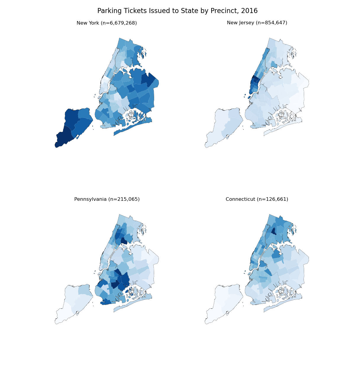
Choropleth of parking tickets issued to state by precinct in NYC

This example plots a subset of parking tickets issued to drivers in New York City. Specifically, it plots the subset of tickets issued in the city which are more common than average for that state than the average. This difference between “expected tickets issued” and “actual tickets issued” is interesting because it shows which areas visitors driving into the city from a specific state are more likely visit than their peers from other states.

Observations that can be made based on this plot include:

• Only New Yorkers visit Staten Island.

• Drivers from New Jersey, many of whom likely work in New York City, bias towards Manhattan.

• Drivers from Pennsylvania and Connecticut bias towards the borough closest to their state: The Bronx for Connecticut, Brooklyn for Pennsylvania.

This example was inspired by the blog post “Californians love Brooklyn, New Jerseyans love Midtown: Mapping NYC’s Visitors Through Parking Tickets”.

Out:

Text(0.5, 1.0, 'Connecticut (n=126,661)')

import geopandas as gpd
import geoplot as gplt
import geoplot.crs as gcrs
import matplotlib.pyplot as plt

# load the data
nyc_boroughs = gpd.read_file(gplt.datasets.get_path('nyc_boroughs'))
tickets = gpd.read_file(gplt.datasets.get_path('nyc_parking_tickets'))

proj = gcrs.AlbersEqualArea(central_latitude=40.7128, central_longitude=-74.0059)


def plot_state_to_ax(state, ax):
    gplt.choropleth(
        tickets.set_index('id').loc[:, [state, 'geometry']],
        hue=state, cmap='Blues',
        linewidth=0.0, ax=ax
    )
    gplt.polyplot(
        nyc_boroughs, edgecolor='black', linewidth=0.5, ax=ax
    )


f, axarr = plt.subplots(2, 2, figsize=(12, 13), subplot_kw={'projection': proj})

plt.suptitle('Parking Tickets Issued to State by Precinct, 2016', fontsize=16)
plt.subplots_adjust(top=0.95)

plot_state_to_ax('ny', axarr[0][0])
axarr[0][0].set_title('New York (n=6,679,268)')

plot_state_to_ax('nj', axarr[0][1])
axarr[0][1].set_title('New Jersey (n=854,647)')

plot_state_to_ax('pa', axarr[1][0])
axarr[1][0].set_title('Pennsylvania (n=215,065)')

plot_state_to_ax('ct', axarr[1][1])
axarr[1][1].set_title('Connecticut (n=126,661)')