Working with Projections

This section of the tutorial discusses map projections. If you don’t know what a projection is, or are looking to learn more about how they work in geoplot, this page is for you!

I recommend following along with this tutorial interactively using Binder.

Projection and unprojection

import geopandas as gpd
import geoplot as gplt
%matplotlib inline

# load the example data
contiguous_usa = gpd.read_file(gplt.datasets.get_path('contiguous_usa'))
gplt.polyplot(contiguous_usa)

<matplotlib.axes._subplots.AxesSubplot at 0x11a914208>

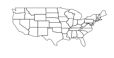
This map is an example of an unprojected plot: it reproduces our coordinates as if they were on a flat Cartesian plane. But remember, the Earth is not a flat surface; it’s a sphere. This isn’t a map of the United States that you’d seen in print anywhere because it badly distorts both of the two criteria most projections are evaluated on: shape and area.

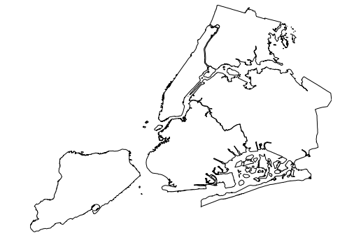
For sufficiently small areas, the amount of distortion is very small. This map of New York City, for example, is reasonably accurate:

boroughs = gpd.read_file(gplt.datasets.get_path('nyc_boroughs'))
gplt.polyplot(boroughs)

<matplotlib.axes._subplots.AxesSubplot at 0x11d243898>

But there is a better way: use a projection.

A projection is a way of mapping points on the surface of the Earth into two dimensions (like a piece of paper or a computer screen). Because moving from three dimensions to two is intrinsically lossy, no projection is perfect, but some will definitely work better in certain case than others.

The most common projection used for the contiguous United States is the Albers Equal Area projection. This projection works by wrapping the Earth around a cone, one that’s particularly well optimized for locations near the middle of the Northern Hemisphere (and particularly poorly for locations at the poles).

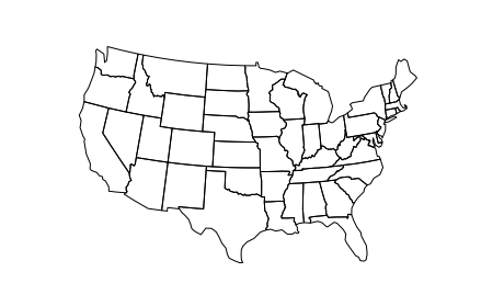
To add a projection to a map in geoplot, pass a geoplot.crs object to the projection parameter on the plot. For instance, here’s what we get when we try Albers out on the contiguous United States:

import geoplot.crs as gcrs
gplt.polyplot(contiguous_usa, projection=gcrs.AlbersEqualArea())

<cartopy.mpl.geoaxes.GeoAxesSubplot at 0x11dd02cc0>

For a list of projections implemented in geoplot, refer to the projections reference in the cartopy documentation (cartopy is the library geoplot relies on for its projections).

Stacking projected plots

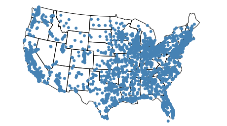
A key feature of geoplot is the ability to stack plots on top of one another.

cities = gpd.read_file(gplt.datasets.get_path('usa_cities'))
ax = gplt.polyplot(
    contiguous_usa,
    projection=gcrs.AlbersEqualArea()
)
gplt.pointplot(cities, ax=ax)

<cartopy.mpl.geoaxes.GeoAxesSubplot at 0x11da21c50>

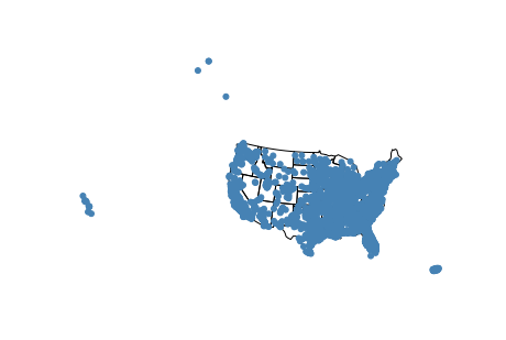
By default, geoplot will set the extent (the area covered by the plot) to the total_bounds of the last plot stacked onto the map.

However, suppose that even though we have data for One entire United States (plus Puerto Rico) we actually want to display just data for the contiguous United States. An easy way to get this is setting the extent parameter using total_bounds.

ax = gplt.polyplot(
    contiguous_usa,
    projection=gcrs.AlbersEqualArea()
)
gplt.pointplot(cities, ax=ax, extent=contiguous_usa.total_bounds)

<cartopy.mpl.geoaxes.GeoAxesSubplot at 0x11da947f0>

The section of the tutorial on Customizing Plots explains the extent parameter in more detail.

Projections on subplots

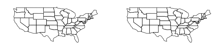
It is possible to compose multiple axes together into a single panel figure in matplotlib using the subplots feature. This feature is highly useful for creating side-by-side comparisons of your plots, or for stacking your plots together into a single more informative display.

import matplotlib.pyplot as plt
import geoplot as gplt

f, axarr = plt.subplots(1, 2, figsize=(12, 4))
gplt.polyplot(contiguous_usa, ax=axarr[0])
gplt.polyplot(contiguous_usa, ax=axarr[1])

<matplotlib.axes._subplots.AxesSubplot at 0x11dc55438>

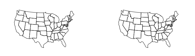
matplotlib supports subplotting projected maps using the projection argument to subplot_kw.

proj = gcrs.AlbersEqualArea(central_longitude=-98, central_latitude=39.5)
f, axarr = plt.subplots(1, 2, figsize=(12, 4), subplot_kw={
    'projection': proj
})
gplt.polyplot(contiguous_usa, projection=proj, ax=axarr[0])
gplt.polyplot(contiguous_usa, projection=proj, ax=axarr[1])

<cartopy.mpl.geoaxes.GeoAxesSubplot at 0x11ded2b70>

The Gallery includes several demos, like the Pointplot Scale Functions demo, that use this feature to good effect.

Notice that in this code sample we specified some additional parameters for our projection. The central_longitude=-98 and central_latitude=39.5 parameters set the “center point” around which the points and shapes on the map are reprojected (in this case we use the geographic center of the contiguous United States).

When you pass a projection to a geoplot function, geoplot will infer these values for you. But when passing the projection directly to matplotlib you must set them yourself.