Gradient Checkpoints
Contents
Gradient Checkpoints
In this chapter we will cover gradient checkpointing. In a nutshell, gradient checkpointing works by recomputing the intermediate values of a deep neural net (which would ordinarily be stored at forward time) at backward time. This enables training larger models and/or larger batch sizes by trading compute (the time cost of recalculating these values twice) for memory (the bandwidth cost of storing these values ahead of time).
At the end of this article, we’ll see an example benchmark showing how gradient checkpointing reduces the model’s memory cost by 60% (at the cost of 25% greater training time).
To follow along in code, check out the GitHub repository.
TLDR: gradient checkpointing allows you to scale single-machine model training to larger models and/or batch sizes without resorting to more invasive techniques like distributed training. It’s a good candidate for squeezing the last bit of computational juice out of your existing setup.
How neural networks use memory
In order to understand how gradient checkpointing helps, we first need to understand a bit about how model memory allocation works.
The total memory used by a neural network is basically the sum of two components.
The first component is the static memory used by the model. Though there is some fixed cost built into a PyTorch model, the cost is totally almost totally dominated by the model weights. The modern deep learning models used in production today have anywhere between 1 million and 1 billion total parameters. For reference, 100-150 million parameters is about the practical limit for an NVIDIA T4 with 16 GB of GPU memory.
The second component is the dynamic memory taken up by the model. Every forward pass through a neural network in train mode computes an activation for every neuron in the network; this value is then stored in the so-called computation graph. One value must be stored for every single training sample in the batch, so this adds up quickly. The total cost is determined by model size and batch size, and sets the limit on the maximum batch size that will fit into your GPU memory.
To learn more about PyTorch autograd, check out PyTorch autograd explained.
How gradient checkpointing helps
Large models are expensive in both the static and dynamic dimensions. They are hard to fit onto the GPU in the first place and hard to train once you get them onto the device because they force a batch size that’s too small to converge.
Various techniques exist to ameliorate one or both of these problems. Gradient checkpointing is one of them.
Gradient checkpointing works by omitting some of the activation values from the computational graph. This reduces the memory used by the computational graph, reducing memory pressure overall (and allowing larger batch sizes in the process).
However, the reason that the activations are stored in the first place is that they are needed when calculating the gradient during backpropagation. Omitting them from the computational graph forces PyTorch to recalculate these values wherever they appear, slowing down computation overall.
Thus, gradient checkpointing is an example of one of the classic tradeoffs in computer science—between memory and compute.
PyTorch provides gradient checkpointing via torch.utils.checkpoint.checkpoint and torch.utils.checkpoint.checkpoint_sequential, which implements this feature as follows (per the notes in the docs). During the forward pass, PyTorch saves the input tuple to each function in the model. During backpropagation, the combination of input tuple and function is recalculated for each function in a just-in-time manner, plugged into the gradient formula for each function that needs it, and then discarded. The net computation cost is roughly that of forward propagating each sample through the model twice.
Gradient checkpointing was first published in the 2016 paper Training Deep Nets With Sublinear Memory Cost. The paper makes the claim that the gradient checkpointing algorithm reduces the dynamic memory cost of the model from O(n) (where n is the number of layers in the model) to O(sqrt(n)), and demonstrates this experimentally by compressing an ImageNet variant from 48 GB to 7 GB in memory.
Testing out the API
There are two different gradient checkpointing methods in the PyTorch API, both in the torch.utils.checkpoint namespace. The simpler of the two, checkpoint_sequential, is constrained to sequential models (e.g. models using the torch.nn.Sequential wrapper); checkpoint, is its more flexible counterpart, can be used for any module.
Here is a complete code sample (taken from an old tutorial) showing checkpoint_sequential in action:
import torch
import torch.nn as nn

from torch.utils.checkpoint import checkpoint_sequential

# a trivial model
model = nn.Sequential(
    nn.Linear(100, 50),
    nn.ReLU(),
    nn.Linear(50, 20),
    nn.ReLU(),
    nn.Linear(20, 5),
    nn.ReLU()
)

# model input
input_var = torch.randn(1, 100, requires_grad=True)

# the number of segments to divide the model into
segments = 2

# finally, apply checkpointing to the model
# note the code that this replaces:
# out = model(input_var)
out = checkpoint_sequential(modules, segments, input_var)

# backpropagate
out.sum().backwards()
As you can see, checkpoint_sequential is a replacement for the forward or __call__ method on the module object. out is almost the same tensor we’d get if we’d called model(input_var); the key differences are that it’s missing accumulated values, and has some extra metadata attached to it instructing PyTorch to recompute these values when it needs them during out.backward().
Notably, checkpoint_sequential takes a segment’s integer value as input. checkpoint_sequential works by splitting the model into n lengthwise segments, and applying checkpointing to each segment except the last.
This is simple and easy to work with, but has some major limitations. You have no control over where the boundaries of the segments are, and there is no way to checkpoint the entire module (instead of some part of it).
The alternative is using the more flexible checkpoint API. To demonstrate, consider the following simple convolutional model:
class CIFAR10Model(nn.Module):
    def __init__(self):
        super().__init__()
        self.cnn_block_1 = nn.Sequential(*[
            nn.Conv2d(3, 32, 3, padding=1),
            nn.ReLU(),
            nn.Conv2d(32, 64, 3, padding=1),
            nn.ReLU(),
            nn.MaxPool2d(kernel_size=2)
        ])
        self.dropout_1 = nn.Dropout(0.25)
        self.cnn_block_2 = nn.Sequential(*[
            nn.Conv2d(64, 64, 3, padding=1),
            nn.ReLU(),
            nn.Conv2d(64, 64, 3, padding=1),
            nn.ReLU(),
            nn.MaxPool2d(kernel_size=2)
        ])
        self.dropout_2 = nn.Dropout(0.25)
        self.flatten = lambda inp: torch.flatten(inp, 1)
        self.linearize = nn.Sequential(*[
            nn.Linear(64 * 8 * 8, 512),
            nn.ReLU()
        ])
        self.dropout_3 = nn.Dropout(0.5)
        self.out = nn.Linear(512, 10)

    def forward(self, X):
        X = self.cnn_block_1(X)
        X = self.dropout_1(X)
        X = torch.utils.checkpoint.checkpoint(self.cnn_block_2, X)
        X = self.dropout_2(X)
        X = self.flatten(X)
        X = self.linearize(X)
        X = self.dropout_3(X)
        X = self.out(X)
        return X
This model has two convolutional blocks, some dropout, and a linear head (the 10 outputs correspond with the 10 classes in CIFAR10).
Here is an updated version of this model using gradient checkpointing:
class CIFAR10Model(nn.Module):
    def __init__(self):
        super().__init__()
        self.cnn_block_1 = nn.Sequential(*[
            nn.Conv2d(3, 32, 3, padding=1),
            nn.ReLU(),
            nn.Conv2d(32, 64, 3, padding=1),
            nn.ReLU(),
            nn.MaxPool2d(kernel_size=2)
        ])
        self.dropout_1 = nn.Dropout(0.25)
        self.cnn_block_2 = nn.Sequential(*[
            nn.Conv2d(64, 64, 3, padding=1),
            nn.ReLU(),
            nn.Conv2d(64, 64, 3, padding=1),
            nn.ReLU(),
            nn.MaxPool2d(kernel_size=2)
        ])
        self.dropout_2 = nn.Dropout(0.25)
        self.flatten = lambda inp: torch.flatten(inp, 1)
        self.linearize = nn.Sequential(*[
            nn.Linear(64 * 8 * 8, 512),
            nn.ReLU()
        ])
        self.dropout_3 = nn.Dropout(0.5)
        self.out = nn.Linear(512, 10)

    def forward(self, X):
        X = self.cnn_block_1(X)
        X = self.dropout_1(X)
        X = checkpoint(self.cnn_block_2, X)
        X = self.dropout_2(X)
        X = self.flatten(X)
        X = self.linearize(X)
        X = self.dropout_3(X)
        X = self.out(X)
        return X
checkpoint, appearing here in forward, takes a module (or any callable, such as a function) and its arguments as input. The arguments will be memoized at forward time, then used to recompute its output value at backward time.
There are some additional changes we had to make to the model definition to make this work.
First of all, you’ll notice that we removed the nn.Dropout layers from the convolutional blocks; this is because checkpointing is incompatible with dropout (recall that effectively runs the sample through the model twice—dropout would arbitrarily drop different values in each pass, producing different outputs). Basically, any layer that exhibits non-idempotent behavior when rerun shouldn’t be checkpointed (nn.BatchNorm is another example). The solution is to refactor the module so the problem layer is not excluded from the checkpoint segment, which is exactly what we did here.
Second, you’ll notice that we used checkpoint on the second convolutional block in the model, but not the first. This is because checkpoint naively determines whether its input function requires gradient descent (e.g. whether it is in no_grad=True or no_grad=False mode) by examining the no_grad behavior of the input tensor. The input tensor to the model is almost always in no_grad=False mode, because we’re almost always interested in calculating the gradient relative to the network weights, not the values of the input sample itself. As a result, checkpointing the first submodule in the model would achieve less than nothing: it would effectively freeze the existing weights in place, preventing them from training at all. Refer to this PyTorch forum thread for some more details.
There are some other probably minor details having to do with RNG state and incompatibility with detached tensors discussed in the docs.
You can see the full training loops for this code sample here and here.
Benchmarks
As a quick benchmark, I enabled model checkpointing on tweet-sentiment-extraction, a sentiment classifier model with a BERT backbone based on Twitter data. You can see that code here. transformers helpfully already implements model checkpointing as an optional part of its API; enabling it for our model is as simple as flipping a single boolean flag:
# code from model_5.py

cfg = transformers.PretrainedConfig.get_config_dict("bert-base-uncased")[0]
cfg["output_hidden_states"] = True
cfg["gradient_checkpointing"] = True  # NEW!
cfg = transformers.BertConfig.from_dict(cfg)
self.bert = transformers.BertModel.from_pretrained(
    "bert-base-uncased", config=cfg
)
I used Spell to train this model four times: once each on an NVIDIA T4 and NVIDIA V100 GPU, and once each in checkpointed and uncheckpointed modes. All runs had a batch size of 64. Here are the results:
Author note: these benchmarks were last run in April 2021.
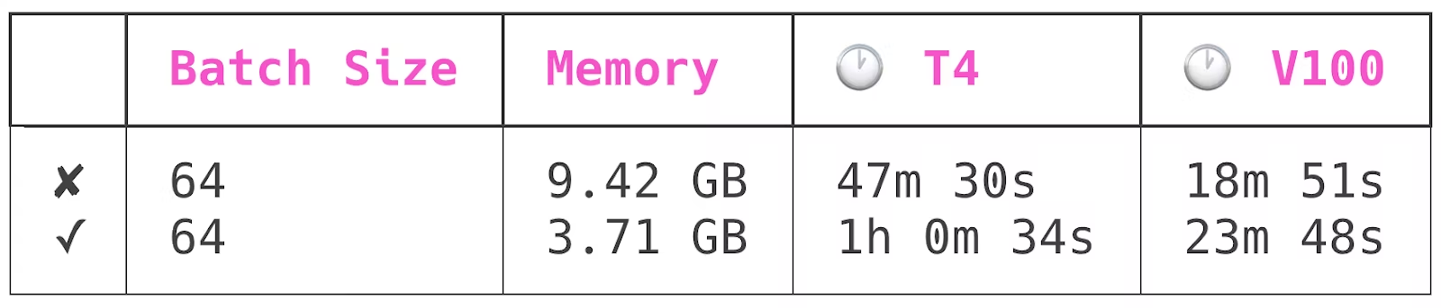
The first row has training runs conducted with model checkpointing off, the second with it on.
Model checkpointing reduced peak model memory usage by about 60%, while increasing model training time by about 25%.
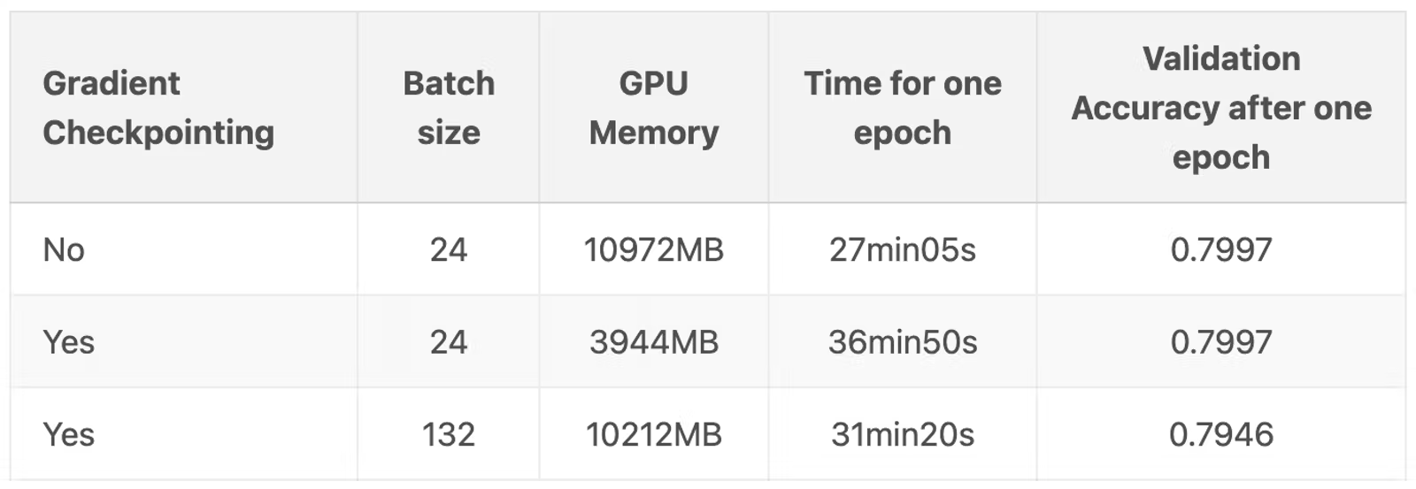
Of course, the primary reason you would want to use checkpoints is so that you can get batch sizes onto GPU that are too large to fit straight up. In the blog post Explore Gradient-Checkpointing in PyTorch, Qingyang Wu demonstrates this by going from 24 to an amazing 132 samples per batch!