Mixed Precision
Contents
Mixed Precision
Mixed-precision training is a technique for substantially reducing neural net training time by performing as many operations as possible in half-precision floating point, fp16, instead of the (PyTorch default) single-precision floating point, fp32. Recent generations of NVIDIA GPUs come loaded with special-purpose tensor cores specially designed for fast fp16 matrix operations.
PyTorch 1.6 added API support for mixed-precision training, including automatic mixed-precision training. Using these cores had once required writing reduced precision operations into your model by hand. Today the torch.cuda.amp API can be used to implement automatic mixed precision training and reap the huge speedups it provides in as few as five lines of code!
TLDR: the torch.cuda.amp mixed-precision training module provides speed-ups of 50-60% in large model training jobs.
How mixed precision works
Before we can understand how mixed precision training works, we first need to review a little bit about floating point numbers.
In computer engineering, decimal numbers like 1.0151 or 566132.8 are traditionally represented as floating point numbers. Since we can have infinitely precise numbers (think π), but limited space in which to store them, we have to make a compromise between precision (the number of decimals we can include in a number before we have to start rounding it) and size (how many bits we use to store the number).
The technical standard for floating point numbers, IEEE 754 (for a deep dive I recommend the PyCon 2019 talk Floats are Friends: making the most of IEEE754.00000000000000002), sets the following standards:
fp64, aka double-precision or “double”, max rounding error of~2^-52fp32, aka single-precision or “single”, max rounding error of~2^-23fp16, aka half-precision or “half”, max rounding error of~2^-10
Python uses fp64 for the float type. PyTorch, which is much more memory-sensitive, uses fp32 as its default dtype instead.
The basic idea behind mixed precision training is simple: halve the precision (fp32 → fp16), halve the training time.
The hard part is doing so safely.
Notice that the smaller the floating point, the larger the rounding errors it incurs. Any operation performed on a “small enough” floating point number will round the value to zero! This is known as underflowing, and it’s a problem because many to most gradient update values created during backpropogation are extremely small but nevertheless non-zero. Rounding error accumulation during backpropogation can turn these numbers into zeroes or nans; this creates inaccurate gradient updates and prevents your network from converging.
The 2018 ICLR paper Mixed Precision Training found that naively using fp16 everywhere “swallows” gradient updates smaller than 2^-24 in value — around 5% of all gradient updates made by their example network:
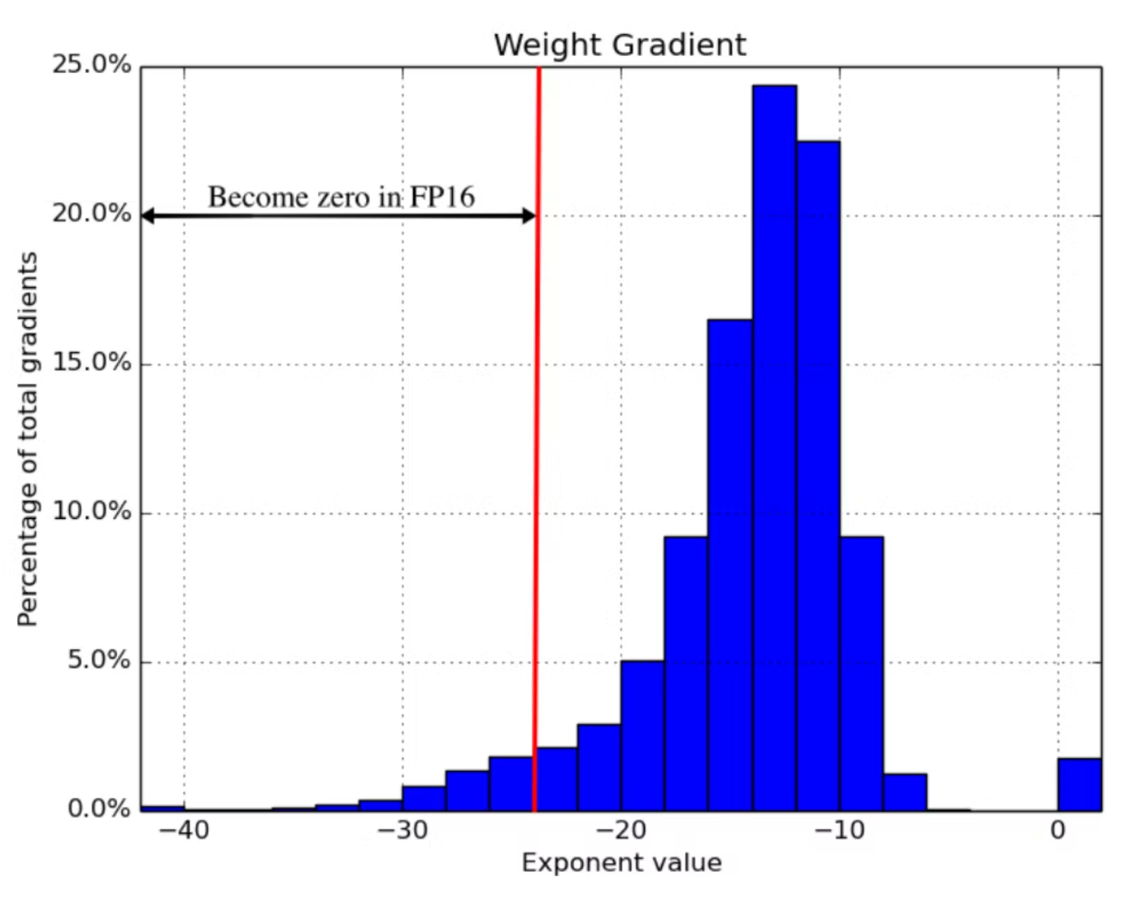
Mixed precision training is a set of techniques which allows you to use fp16 without causing your model training to diverge. It’s a combination of three different techniques.
One, maintain two copies of the weights matrix, a “master copy” in fp32, and a half-precision copy of it in fp16. Gradient updates are calculated using the fp16 matrix but applied to the fp32 matrix. This makes applying the gradient update much safer.
Two, different vector operations accumulate errors at different rates, so treat them differently. Some operations are always safe in fp16, but others are only reliable in fp32. Instead of running the entire neural network in fp16, run some parts in halves and others in singles. This mixture of dtypes is why this technique is called “mixed precision”.
Three, use loss scaling. Loss scaling means multiplying the output of the loss function by some scalar number (the paper suggests starting with 8) before performing back-propagation. Multiplicative increases in the loss values create multiplicative increases in gradient update values, “lifting” many gradient update values above the 2^-24 threshold for fp16 safety. Just make sure to undo the loss scaling before applying the gradient update, and don’t pick a loss scaling so large that it produces inf weight updates (overflowing), causing the network to diverge in the other direction.
Combining these three techniques in tandem allowed the authors to train a variety of networks to convergence in significantly expedited time. For benchmarks, I recommend reading the paper — it’s only 9 pages long!
How tensor cores work
While mixed precision training saves memory everywhere (an fp16 matrix is half the size of a fp32 one), it doesn’t provide a model training speedup without special GPU support. There needs to be something on the chip that accelerates half-precision operations. In recent generations of NVIDIA GPUs, there is: tensor cores.
Tensor cores are a new type of processing unit that’s optimized for a single very specific operation: multiplying two 4 x 4 fp16 matrices together and adding the result to a third 4 x 4 fp16 or fp32 matrix (a “fused multiply add”).
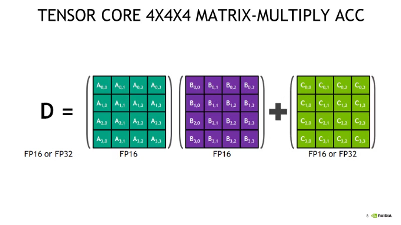
Larger fp16 matrix multiplication operations can be implemented using this operation as their basic building block. And since most of backpropagation boils down to matrix multiplication, tensor cores are applicable to almost any computationally intensive layer in the network.
The catch: the input matrices must be in fp16. If you’re training on a GPU with tensor cores and not using mixed precision training, you’re not getting 100% out of your card! A standard PyTorch model defined in fp32 will never land any fp16 math onto the chip, so all of those sweet, sweet tensor cores will remain idle.
Tensor cores were introduced in late 2017 in the last-gen Volta architecture, saw improvement in current-gen Turing, and will see further refinements in the still-forthcoming Ampere. The two GPUs generally available on the cloud that support are the V100 (5120 CUDA cores, 600 tensor cores) and the T4 (2560 CUDA cores, 320 tensor cores).
One other piece of the puzzle worth keeping in mind is firmware. Although all versions of CUDA 7.0 or higher supports tensor core operations, early implementations are reputedly very buggy, so it’s important to be on CUDA 10.0 or higher.
How PyTorch automatic mixed precision works
With that important background out of the way, we’re finally ready to dig into the new PyTorch amp API.
Mixed precision training has technically been possible forever: run sections of your network in fp16 manually and implement loss scaling yourself. The exciting thing in automatic mixed-precision training is the “automatic” part. There’s just a couple of new API primitives to learn: torch.cuda.amp.GradScalar and torch.cuda.amp.autocast. Enabling mixed precision training is as simple as slotting these into the right places in your training script!
To demonstrate, here’s an excerpt of the training loop for a network using mixed-precision training. # NEW marks spots where new code got added.
self.train()
X = torch.tensor(X, dtype=torch.float32)
y = torch.tensor(y, dtype=torch.float32)

optimizer = torch.optim.Adam(self.parameters(), lr=self.max_lr)
scheduler = torch.optim.lr_scheduler.OneCycleLR(
    optimizer, self.max_lr,
    cycle_momentum=False,
    epochs=self.n_epochs,
    steps_per_epoch=int(np.ceil(len(X) / self.batch_size)),
)
batches = torch.utils.data.DataLoader(
    torch.utils.data.TensorDataset(X, y),
    batch_size=self.batch_size, shuffle=True
)

# NEW
scaler = torch.cuda.amp.GradScaler()

for epoch in range(self.n_epochs):
    for i, (X_batch, y_batch) in enumerate(batches):
        X_batch = X_batch.cuda()
        y_batch = y_batch.cuda()
        optimizer.zero_grad()

        # NEW
        with torch.cuda.amp.autocast():
            y_pred = model(X_batch).squeeze()
            loss = self.loss_fn(y_pred, y_batch)

        # NEW
        scaler.scale(loss).backward()
        lv = loss.detach().cpu().numpy()
        if i % 100 == 0:
            print(f"Epoch {epoch + 1}/{self.n_epochs}; Batch {i}; Loss {lv}")

        # NEW
        scaler.step(optimizer)
        scaler.update()

        scheduler.step()
The new PyTorch GradScaler object is PyTorch’s implementation of loss scaling. Recall from the section “How mixed precision works” that some form of loss scaling is necessary to keep gradients from rounding down to 0 during training. The optimal loss multiplier is one sufficiently high to retain very small gradients, but not so high that it causes very large gradients to round up to inf, creating the opposite problem.
However, there is no one loss multiplier that will work for every network. The optimal multiplier is also very likely to change over time, as gradients are typically much larger at the start of training than at the end. How do you find the optimal loss multiplier without giving the user another hyperparameter that they have to tune?
PyTorch uses exponential backoff to solve this problem. GradScalar starts with a small loss multiplier, which every so often it doubles. This gradual doubling behavior continues until GradScalar encounters a gradient update containing inf values. GradScalar discards this batch (e.g. the gradient update is skipped), halves the loss multiplier, and resets its doubling cooldown.
Stepping the loss multiplier up and down in this way allows PyTorch to approximate the appropriate loss multiplier over time. Readers familiar with TCP congestion control should find the core ideas here very familiar! The exact numbers used by the algorithm are configurable, and you can read the defaults right out of the docstring:
torch.cuda.amp.GradScaler(
    init_scale=65536.0, growth_factor=2.0, backoff_factor=0.5,
    growth_interval=2000, enabled=True
)
GradScalar needs to exert control over the gradient update calculations (to check for overflow) and over the optimizer (to turn discarded batches into a no-op) to implement its behavior. This is why loss.backwards() is replaced with scaler.scale(loss).backwards() and optimizer.step() is replaced with scaler.step(optimizer).
It’s notable that GradScalar will detect and stop overflows (because inf is always bad), but it has no way to detect and stop underflows (because 0 is often a legitimate value). If you pick an init_scale that’s too low and a growth_interval that’s too high, your network may underflow and diverge before GradScalar can intervene. For this reason it’s probably a good idea to pick a very large starting value, and with default init_scale=65536 (2¹⁶) that does seem to be the approach that PyTorch is following.
Finally, note that GradScalar is a stateful object. Checkpointing a model using this feature will require writing it to and reading it from disk in alongside your model weights. This is easy to do using the state_dict and load_state_dict object methods (covered here in the PyTorch docs).
The other half of the automatic mixed-precision training puzzle is the torch.cuda.amp.autocast context manager. Autocast implements fp32 -> fp16 behavior. Recall from “How mixed precision works” that, because different operations accumulate errors at different rates, not all operations are safe to run in fp16. The following screenshots taken from the amp module documentation covers how autocast treats the various operations available in PyTorch:
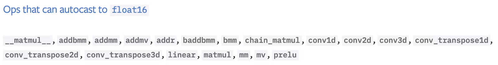
This list predominantly consists of two things, matrix multiplication and convolutions. The simple linear function is also present.
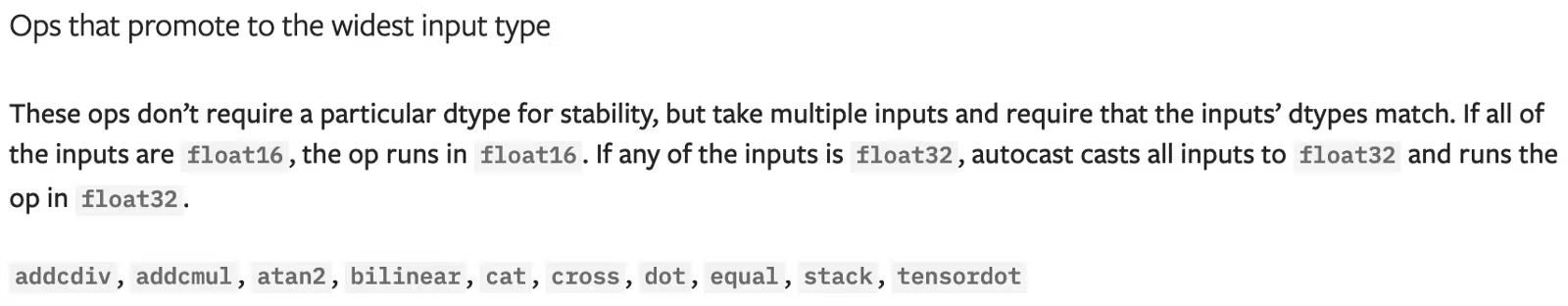
These operations are safe in fp16, but have up-casting rules to ensure that they don’t break when given a mixture of fp16 and fp32 input. Note that this list includes two other fundamental linear algebraic operations: matrix/vector dot products and vector cross products.
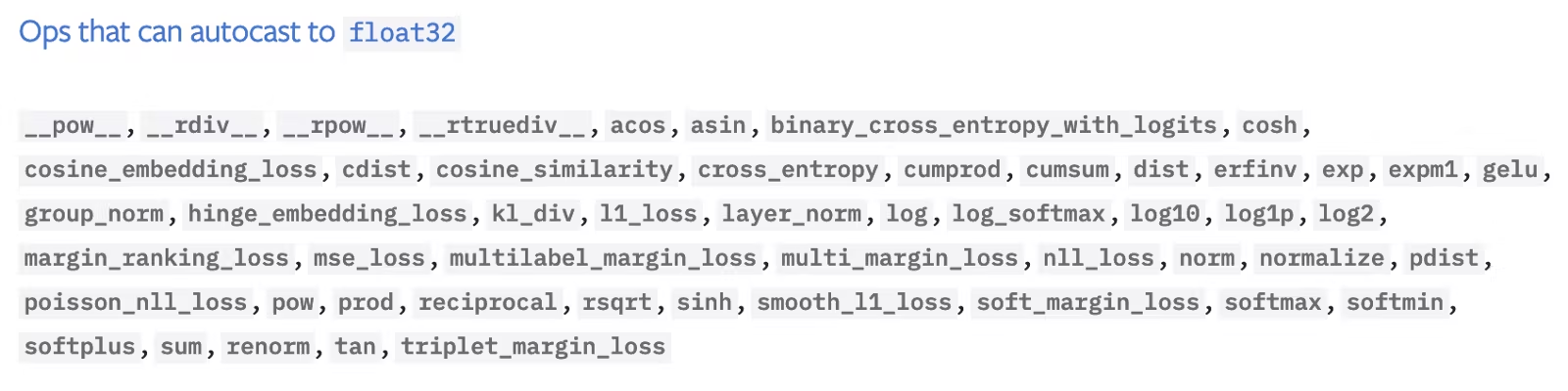
Logarithms, exponents, trigonometric functions, normal functions, discrete functions, and (large) sums are unsafe in fp16 and must be performed in fp32.
Looking through the list, it seems to me that most layers would benefit from autocasting, thanks to their internal reliance on fundamental linear algebra operations, but most activation functions would not. Convolutional layers stand out as potentially the biggest winner.
Enabling autocasting is dead simple. All you need to do is wrap the forward pass of your model using the autocast context manager:
with torch.cuda.amp.autocast():
    y_pred = model(X_batch).squeeze()
    loss = self.loss_fn(y_pred, y_batch)
Wrapping the forward pass in this way automatically enables autocasting on the backwards pass (e.g. loss.backwards()) as well, so you don’t need to call autocast twice.
So long as you follow best practices for using PyTorch (avoiding in-place operations, for example), autocasting basically “just works”. It even works out-of-the-box with the multi-GPU DistributedDataParallel API (so long as you follow the recommended strategy of using one process per GPU). It works with the DataParallel multi-GPU API too, with one small adjustment. The “Working with multiple GPUs” section of the Automatic Mixed Precision Examples page in the PyTorch docs is a handy reference on this subject. The one major “gotcha” (IMO) to keep in mind: “prefer binary cross entropy with logits over binary cross entropy”.
Performance benchmarks
At this point we’ve learned what mixed precision is, what tensor cores are, and how the PyTorch API implementing automatic mixed precision behaves. The only thing left is looking at some real-world performance benchmarks!
I trained three very different neural networks once with automatic mixed precision and once without, using V100s (last-gen tensor cores) and T4s (current-gen tensor cores) via the Spell API. I used AWS EC2 instances, p3.2xlarge and g4dn.xlarge respectively, a recent PyTorch 1.6 nightly, and CUDA 10.0. All of the models converged equally, e.g. none of the models saw any difference in training loss between the mixed precision and vanilla network. The networks trained were:
Feedforward, a feedforward neural network trained on data from the Rossman Store Samples competition on Kaggle. Get the code here.UNet, a medium-sized vanilla UNet image segmentation net trained on the Segmented Bob Ross Images corpus. Get the code here.BERT, a large NLP transformer model using thebert-base-uncasedmodel backbone (viahuggingface) and data from the Twitter Sentiment Extraction competition on Kaggle. Get the code here.
The results:
Author note: these benchmarks were last run in June 2020. Improvements in the implementation have likely reduced training times even further since then.
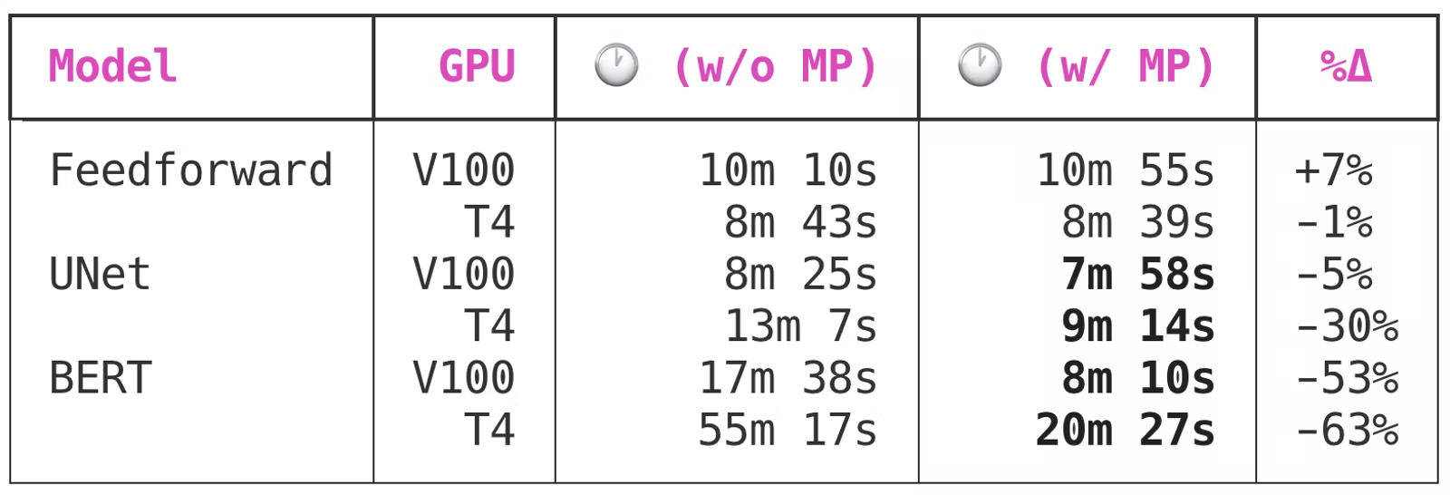
Because the feedforward network is very small, it gets no benefit from mixed precision training.
UNet, a medium-sized convolutional model with 7,703,497 total parameters, sees significant benefits from enabling mixed precision training. Interestingly, though the V100 and T4 both benefit from mixed precision training, the benefit to the T4 is much greater: a 5% time save versus a whopping 30% time save.
BERT is a large model, and it’s where the time savings of using mixed precision training go from “nice” to “must-have”. Automatic mixed precision will cut training time for large models trained on Volta or Turing GPU by 50 to 60 percent! 🔥
This is a huge, huge benefit, especially when you take into account the minimal complexity required — just four or five LOC to your model training script. In my opinion:
Mixed precision should be one of the first performance optimization you make to your model training scripts.
What about memory?
As I explained in the section “How mixed precision works”, an fp16 matrix is half the size of a fp32 matrix in memory, so another purported advantage of mixed precision training is memory usage. GPU memory is much less of a bottleneck than GPU compute, but it’s still pretty valuable to optimize. The more efficient your memory usage, the larger the batch sizes you can fit on the GPU.
PyTorch reserves a certain amount of GPU memory at the beginning of the model training process and holds onto that memory for the duration of the training job. This keeps other processes from reserving too much GPU memory mid-training, forcing the PyTorch training script to crash with an OOM error.
Here is the impact that enabling mixed precision training has on the PyTorch memory reservation behavior:
Author note: these benchmarks were last run in June 2020.
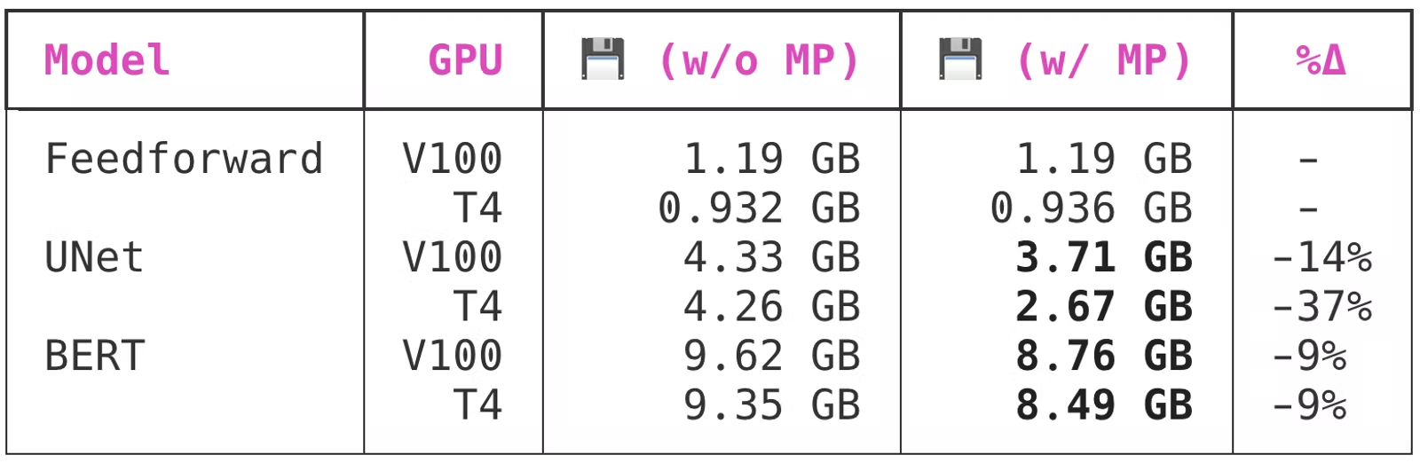
Interestingly enough, while both of the larger models saw benefit from the swap to mixed precision, UNet benefited from the swap a lot more than BERT did. PyTorch memory allocation behavior is pretty opaque to me, so I have no insight into why this might be the case.
To learn more about mixed precision training directly from the source, see the automatic mixed precision package and automatic mixed precision examples pages in the PyTorch docs.