Assorted Tricks
Contents
Assorted Tricks
The chapter covers miscellaneous commonly used model training “tricks”. By “tricks” I mean simple techniques that are straightforward to implement (in a few lines of code at most) and explain.
This section currently has eight different “tricks”, presented in no particular order.
Use pinned memory for data loading
TLDR: as long as your machine has enough RAM to comfortably fit each batch of data onto your machine, enable memory pinning on your data batches to speed up batch loading. This can provide a sigificant performance boost to I/O-bound model training runs.
A page is an atomic unit of memory in OS-level virtual memory management. The de-facto “standard” page size is 4 KiB, though recent operating systems and hardware platforms often support larger sizes.
Paging is the act of storing and retrieving memory pages from disk (HDD or SSD) to main memory (RAM). Paging is used to allow the working memory set of the applications running on the OS to exceed the total RAM size. If you’ve ever opened a resource browser utility on a machine with (say) 16 GB of RAM, and seen it say you’re currently using 20 GB, that’s paging at work. 4 of those 20 GB got spilled to disk.
Non-paged memory is memory that is in RAM, e.g. it has not been spilled to disk. You may tell your OS (using the CUDA API) to never spill certain pages to disk. In CUDA lexicon, this is referred to as pinning, and it results in pinned memory. Pinned memory is guaranteed to be non-paged.
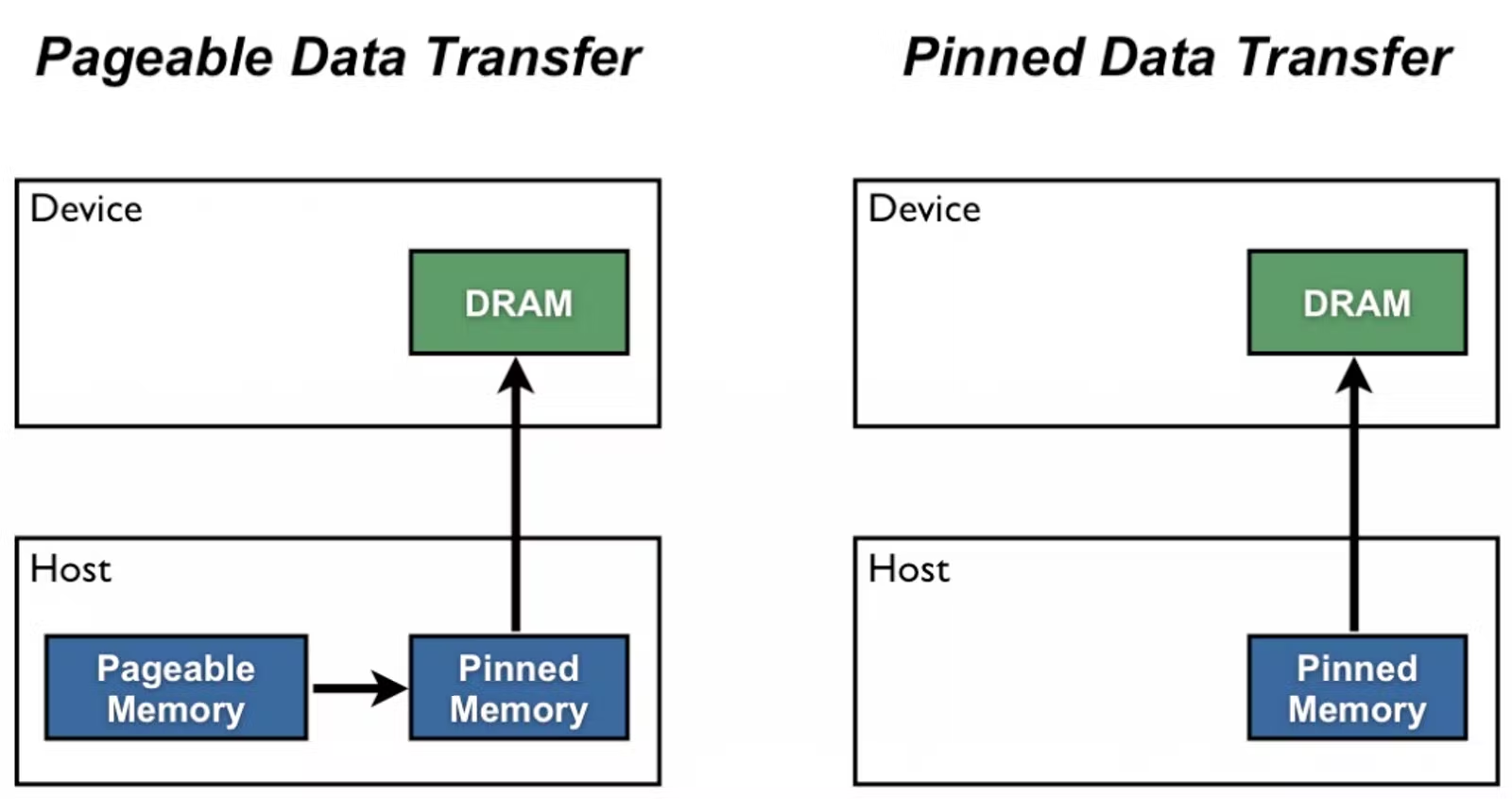
Pinned memory is used to speed up a CPU to GPU memory copy operation (as executed by tensor.cuda() in PyTorch) by guaranteeing that all of the data is in RAM, not spilled to permanent storage. Memory cached to disk has to first be read into RAM before it can be transferred to the GPU, resulting in a disk seek and a double copy, which slows the operation down. The following diagram, taken from this blog post, illustrates:

PyTorch supports pinning batch data using the pin_memory field (pin_memory=True) on DataLoader. This feature is documented here in the PyTorch docs.
Keep in mind that this technique requires the OS to give the PyTorch process as much main memory as it needs to complete its load and transform operations. The batch must fit into RAM, in its entirety, without starving the rest of the machine of resources!
Use multiprocessing for data loading
TLDR: the PyTorch DataLoader processes data on a single process by default. It is almost always better to use its num_workers feature to split data processing across multiple processes instead. As a rule of thumb, you should use four times as many processes as you have GPUs.
DataLoader by default loads and transforms data in a single process. However, the work it does loading and transforming batches of data is embarrassingly parallel. We can speed things up by parallelizing the work somehow.
In CPU workloads, parallelizing code means using either multithreading, which distributes the work amongst multiple threads on a single processes, or multiprocessing, which distributes the work amongst multiple single-threaded processes. Compute-bounded multithreaded code is famously impractical in Python due to Python’s infamous Global Interpreter Lock.
For this reason DataLoader implements multiprocess parallelization. This is done using the optional num_worker argument. Setting num_workers to any value other than its default 0 will spin up worker processes that individually load and transform the data and load it into the main memory of the host process.
Workers are created whenever an iterator is created from the DataLoader (at __iter__() call time). They are destroyed when StopIterator is reached, or when the iterator is garbage collected. They receive the following objects from the parent (via IPC): the wrapped Dataset object, a worker_int_fn, and a collate_fn. A torch.utils.data.get_worker_info API may be used to write code specific to each worker within these ops.
Data loading via worker processes is trivially easy to do when the root dataset is map type; the parent process will handle assigning the indices of the data to load to the workers. Datasets of an iterator type are harder to work with; you will have to use the APIs above to handle slicing them appropriately. This is documented here in the PyTorch docs.
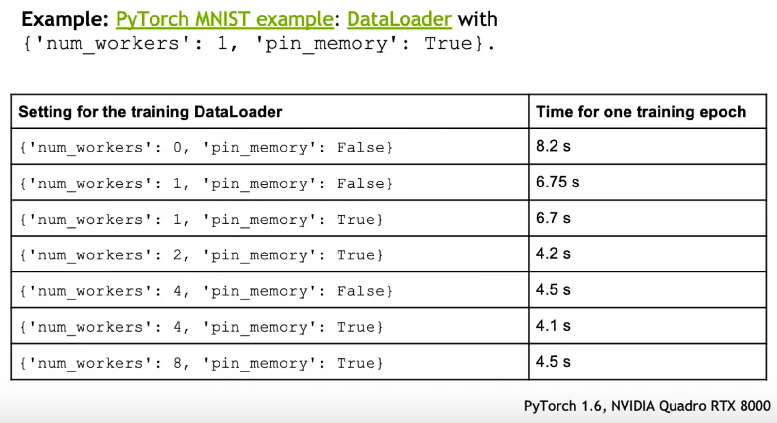
What are the performance benefits of using multiple workers? The PyTorch Performance Tuning Guide talk shows the following benchmarks on a trivial MNIST example (with and without memory pinning, discussed in the previous section):

Use non-blocking device memory transfers
TLDR: most model training scripts involve some amount of work transfering memory from the host to GPU. Making these calls non-blocking by setting non_blocking=True allows you to execute the transfer concurrently with other code, speeding up script runtime.
A code operation is said to be blocking if script execution halts there until it is complete. Blocking code prevents, or “blocks”, any of the lines of codes that comes after it from executing until it is done.
Code that instead executes asynchronously, in parallel with any other code that comes after it, is said to be non-blocking.
PyTorch supports non-blocking memory transfers between devices. To enable this, set the optional non_blocking=True flag on your .to() or .cuda() calls. This memory transfer will run concurrently with the code immediately following this call, unless that code requires access to this tensor’s data, in which case it will block until the transfer is complete.
You can speed up script execution by using placing some other tensor-independent work in your main process immediately after your non-blocking memory transfer calls. For example, this would be the ideal time to make network calls to e.g. wandb.
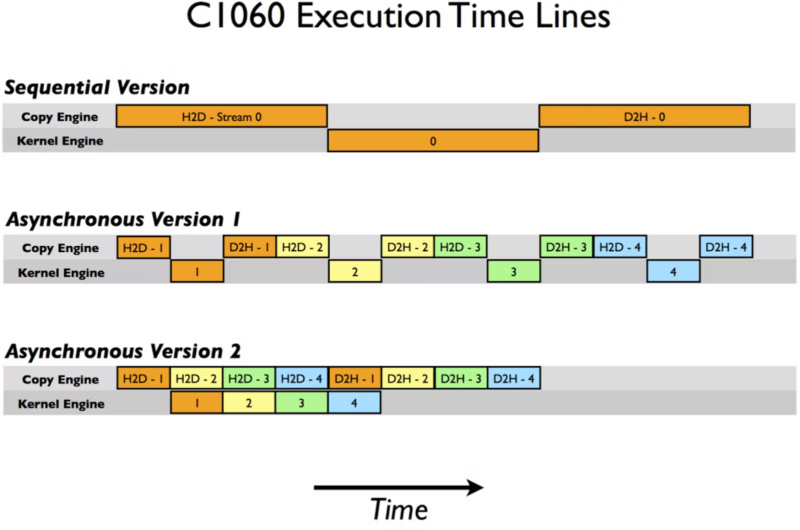
This optimization is particularly important when using pinned memory (if you are not familiar with this concept, refer to the first section of this page for details). Low-level CUDA optimizations explained here on the NVIDIA blog allow certain types of data transfers onto the GPU device from pinned memory only to execute concurrently with GPU kernel processes. Here is a visualization from that blog post that summarizes how it works:

In the first (sequential) example, data loading blocks kernel execution and vice versa. In the latter two (concurrent) examples, the load and execute tasks are first broken down into smaller subtasks, then pipelined in a just-in-time manner.
PyTorch uses this feature to pipeline GPU code execution alongside GPU data transfer:
# assuming the loader call uses pinned memory
# e.g. it was DataLoader(..., pin_memory=True)
for data, target in loader:
    # these two calls are also nonblocking
    data = data.to('cuda:0', non_blocking=True)
    target = target.to('cuda:0', non_blocking=True)
    # model(data) is blocking, so it's a synchronization point
    output = model(data)
In this example, taken from a discuss.pytorch.org thread, model(data) is the first synchronization point. Creating the data and target tensors, moving the data tensor to GPU, and moving the target tensor to GPU, and then performing a forward pass in the model, are pipelined for you by the PyTorch CUDA binding.
The details of how this is done are inscrutable to the end-user. Suffice to say, the end result looks less like Sequential Version and more like Asynchronous Version 2.
Instead of zeroing out the gradient, set it to None
TLDR: recent versions of PyTorch support replacing zero-valued gradients with None values, speeding up backpropagation. The effect on model convergence should be very minimal.
Proceeding with a new batch of training requires clearing out the gradients accumulated thus far. Historically, this has been done by calling model.zero_grad() immediately before calling model(batch). Example code:
for (X, y) in dataloader:
    # zero out gradients, forward prop...
    model.zero_grad()
    y_pred = model(X)

    # ...then back prop.
    loss = loss_fn(y, y_pred)
    loss.backward()
    optimizer.step()
This sets all of the gradients attached to free weights in the model to 0.
PyTorch 1.7 added a new option to zero_grad: model.zero_grad(set_to_none=True). In this mode gradients are initialized with None instead of 0.
Null initialization is slightly more performant than zero initialization for the following reasons:
Zero initialization requires writing a value (
0) to memory, null initialization does not (presumably it creates a bitwise nullity mask instead).Null initialization will change the first update to the gradient value from a “sum” operation (which requires a read-write) to an “assign” operation (which only requires a write), which is slightly faster.
torch.optimoptimizers will still perform a gradient update on gradients with value0. Though some sophisticated optimizers may still calculate a non-zero weight update in this scenario (due to things like annealing, weighted averaging, weight decay) this is usually not very important to model convergence.torch.optimoptimizers completely skipNone-valued gradients, saving time.
Due to the third effect, this parameter is technically not side-effect free. I have never personally experienced a scenario where using model.zero_grad(set_to_none=True) led to divergent behavior, but it seems possible. You can always try turning it off later, to see if it makes a difference.
Turn on cudNN benchmarking
TLDR: cuDNN benchmarking will expedite the training of models making heavy use of convolutional layers by ensuring you use the fastest algorithm for your specific hardware and tensor input shapes.
This optimization is specific to models that make heavy use of convolutional layers (convolutional neural networks and/or model architectures with a convolutional backbone).
Convolutional layers use a well-defined mathematical operation, convolution, which holds foundational importance in a huge variety of applications: image processing, signal processing, statistical modeling, compression, the list goes on and on. As a consequence, a large number of different algorithms have been developed for computing convolutions efficiently on different array sizes and hardware platforms.
PyTorch transitively relies on NVIDIA’s cuDNN framework for the implementations of these algorithms. cuDNN has a benchmarking API, which runs a short program to chose an algorithm for performing convolution which is optimal for the given array shape and hardware.
You can enable benchmarking by setting torch.backends.cudnn.benchmark = True. Thereafter, the first time a convolution of a particular size is run on your GPU device, a fast benchmark program will be run first to determine the best cuDDN convolutional implementation for that given input size is. Thereafter every convolutional operation on a same-sized matrix will use that algorithm instead of the default one.
Again drawing from the PyTorch Performance Tuning Guide talk, we can see the magnitude of the benefit:

Keep in mind that using cudNN benchmarking will only result in a speed if you keep the input size (the shape of the batch tensor you pass to model(batch)) fixed. Otherwise, benchmarking will fire every time input size changes. Deep learning models almost universially use a fixed tensor shape and batch size, so this shouldn’t usually be a concern.
Try using multiple batches per gradient update
TLDR: you can pass multiple batches through a model before backpropagating. This allows you to batch sizes that otherwise wouldn’t fit on the machine, speeding up training times for networks that are bottlenecked by batch size.
Forward propagating some values through a neural network in train mode creates a computational graph that assigns a weight (a gradient) to every free parameter in the model. Backpropagation then adjusts these gradients to more accurate (“better”) values, consuming the computational graph in the process.
However, not every forward pass needs to have a backward pass. In other words, you can call model(batch) as many times as you’d like before you finally call loss.backward(). The computational graph will continue to accumulate gradients until you finally decide to collapse them all.
For models whose performance is bottlenecked by GPU memory, and hence batch size — a lot of NLP models, in particular, have this problem — this simple technique offers an easy way to get a “virtual” batch size larger than will fit in memory.
For example, if you can only fit 16 samples per batch in GPU memory, you can forward pass two batches, then backward pass once, for an effective batch size of 32. Or forward pass four times, backwards pass once, for a batch size of 64. And so on.
The huggingface Training Neural Nets on Larger Batches blog post provides the following code sample illustrating how this works:
model.zero_grad()                                   # Reset gradients tensors
for i, (inputs, labels) in enumerate(training_set):
    predictions = model(inputs)                     # Forward pass
    loss = loss_function(predictions, labels)       # Compute loss function
    loss = loss / accumulation_steps                # Normalize our loss (if averaged)
    loss.backward()                                 # Backward pass
    if (i+1) % accumulation_steps == 0:             # Wait for several backward steps
        optimizer.step()                            # Now we can do an optimizer step
        model.zero_grad()                           # Reset gradients tensors
        if (i+1) % evaluation_steps == 0:           # Evaluate the model when we...
            evaluate_model()                        # ...have no gradients accumulated
Notice that you’ll need to combine the per-batch losses somehow. You can almost always just take the average. For reference, the DistributedDataParallel PyTorch API (covered in a different section of this guide), which does basically this same work, just distributed across multiple machines, is hard-coded to average the gradients.
There’s only one downside to using multiple batches instead of one that I’m aware of. Any fixed costs that occur during training — latency when transferring data between host and GPU memory, for example — will be paid twice.
Use gradient clipping
TLDR: gradient clipping can expedite training of certain kinds of neural networks by clipping unreasonably large gradient updates to a reasonable maximum value.
Gradient clipping is the technique, originally developed for handling exploding gradients in recurrent neural networks, of clipping gradient values that get to be too large to a more realistic maximum value. Basically, you set a max_grad, and PyTorch applies min(max_grad, actual_grad) at backpropagation time (note that this API is bidirectional — a max_grad of 10 will ensure that gradient values fall in the range [-10, 10]).
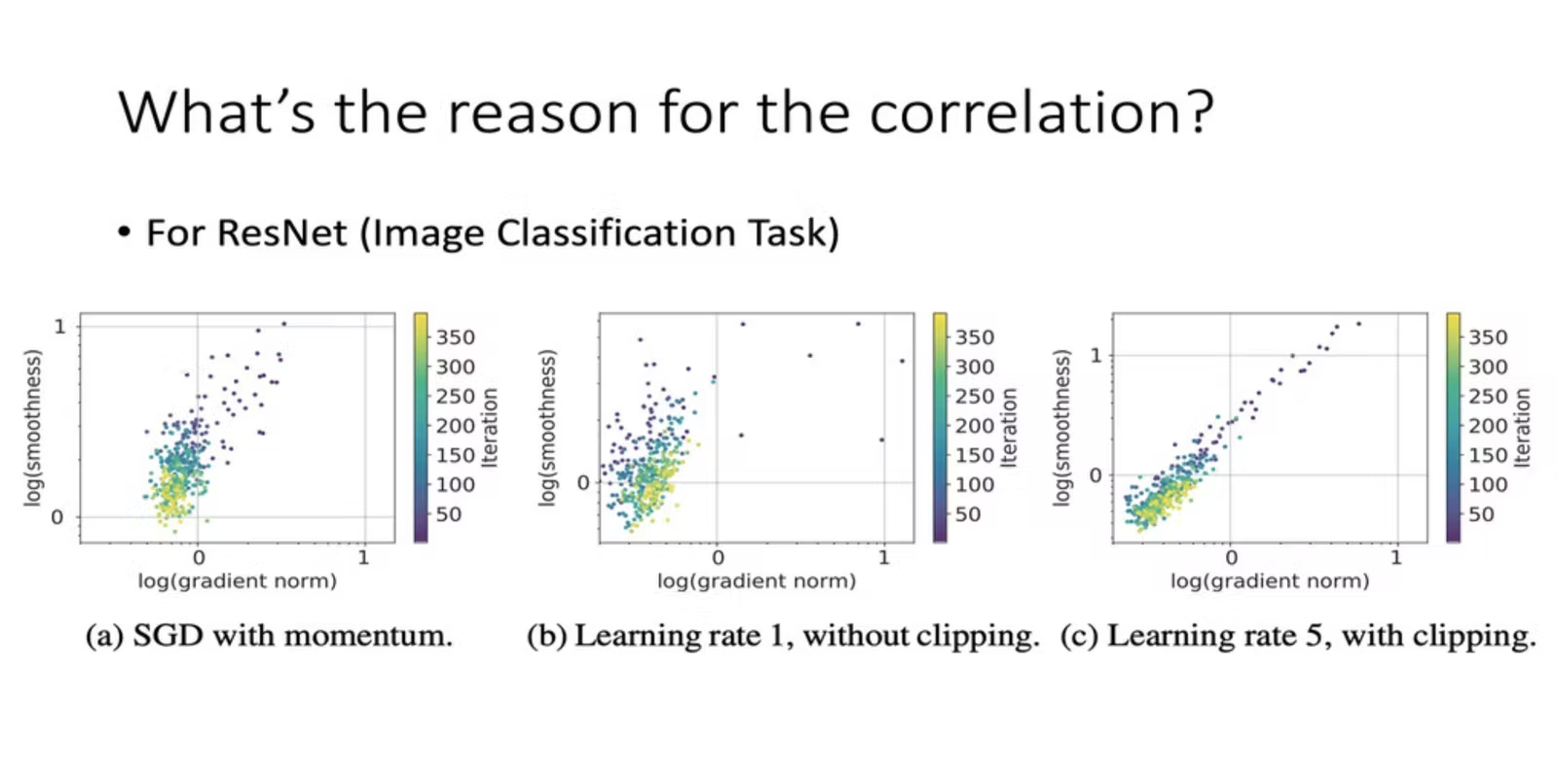
The paper Why Gradient Clipping Accelerates Training: A Theoretical Justification for Adaptivity shows (and provides some theoretical justification for why) gradient clipping can improve convergence behavior, potentially allowing you to choose a higher learning rate (and hence converge to an optimized model more quickly):

Gradient clipping in PyTorch is provided via torch.nn.utils.clip_grad_norm_. You can apply it to individual parameter groups on a case-by-case basis, but the easiest and most common way to use it is to apply the clip to the model as a whole:
torch.nn.utils.clip_grad_norm_(model.parameters(), max_grad)
This code sample is taken directly from the huggingface transformer codebase here.
What should max_grad be set to? Unfortunately, this is not an easy question to answer, as what constitutes a “reasonable” magnitude varies wildly. It’s best to treat this value as another hyperparameter to be tuned. As a rule of thumb, the 2013 paper Generating Sequences With Recurrent Neural Networks used the value 10 for the intermediate layers and 100 for the output head.
Disable bias in convolutional layers before batchnorm
Basically every modern neural network architecture uses some form of normalization, with the OG batch norm being the most common.
PyTorch’s basic batch norm layer (torch.nn.BatchNorm2d) has a bias tensor. If the prior layer (1) also has a bias tensor (2) applied to the same axis as the batch norm bias tensor (3) that is not then squashed by an activation function, the two bias tensors are duplicating work.
In this scenario, it is safe to disable the previous layer’s bias term by passing bias=False at layer initialization time, shaving some parameters off of total model size.
This optimization is most commonly applicable to convolutional layers, which very often use a Conv -> BatchNorm -> ReLU block. For example, here’s a block used by MobileNet with this optimization applied:
nn.Conv2d(hidden_dim, hidden_dim, 3, stride, 1, groups=hidden_dim, bias=False),
nn.BatchNorm2d(hidden_dim),
nn.ReLU6(inplace=True),
Here’s an example block where this optimization doesn’t apply:
nn.Linear(64, 32),
nn.ReLU(),
nn.BatchNorm2d(),
In this case, even though nn.Linear does have a bias term on the same axis as nn.BatchNorm2d, the effect of that term is being squeezed non-linearly by nn.ReLU first, so there is no actual duplication of work.
