Model Pruning
Contents
Model Pruning
This chapter is an introduction to a new idea in deep learning model optimization: model pruning. Model pruning is the technique of reducing the size of a deep learning model by finding small weights in the model and setting them to zero. Model can substantially reduce model size, and may one day speed up model inference time as well.
In this chapter, we will introduce model pruning conceptually: what it is, how it works, and some approaches to using it. We’ll introduce the lottery ticket hypothesis and discuss why the influential paper behind it has led to a resurgence of interest in this topic. Finally, we’ll test out model pruning ourselves in PyTorch, benchmarking it on a demo model that we’ve built (GH repo).
TLDR: although model pruning currently provides significant savings in model artifact size, it does not currently have any effect on model training times due to limitations in PyTorch sparse tensor support. However this will almost certainly change in the future—watch this space!
The basic idea
The basic idea behind model pruning is simple. Deep learning models which have been trained to convergence typically have a large number of weights very close to zero contributing very little weight to model inference. For example, the 2018 ICLR paper Mixed Precision Training includes the following graphic showing weight values in a typical deep neural network (note that “Becomes zero in FP16” is unrelated):
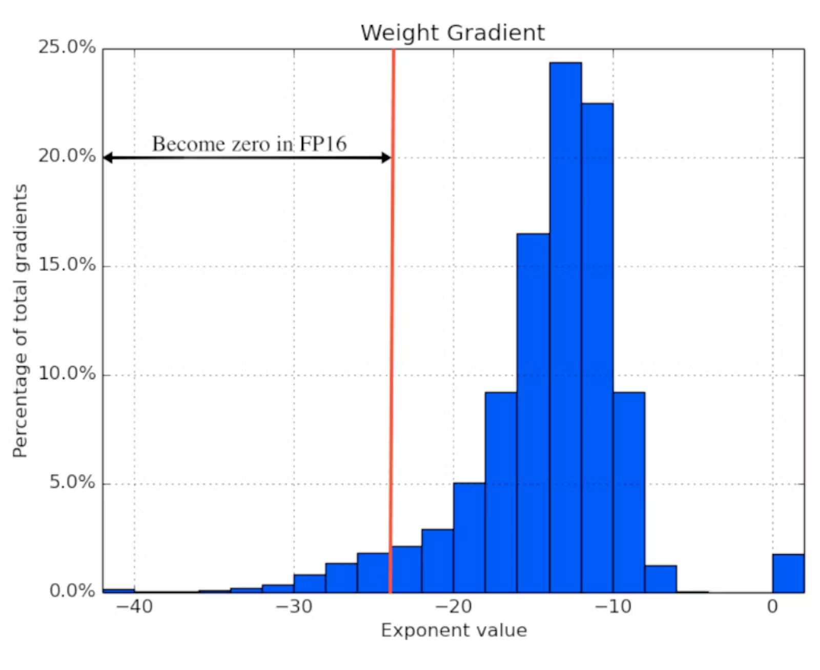
The smaller the weight, the more likely it is that it can be taken to zero without significantly affecting model performance. This same basic idea informed the development of ReLU activation.
However, there are many decisions that need to be made for this to work in practice:
Structure. Unstructured pruning approaches remove weights on a case-by-case basis. Structured pruning approaches remove weights in groups—e.g. removing entire channels at a time. Structured pruning typically has better runtime performance characteristics (it’s a dense computation on fewer channels) but also has a heavier impact on model accuracy (it’s less selective).
Scoring. How do you determine that a weight is small? PyTorch provides three different scoring mechanisms. Random pruning is not very performant, but serves as a useful benchmark. L1 pruning scores weights by measuring their contribution to the overall tensor vector using taxicab distance—e.g. in the weights matrix [[0.01, 0.05], [0.11, 0.12]], the 0.01 value would be pruned first, because it is the component of the vector <0.01, 0.05, 0.11, 0.12> with the smallest magnitude. Finally, you can use any other norm, e.g. L2 (Euclidean distance), using Ln pruning.
Aside: if you are unfamiliar with norms and/or distance metrics, or need a refresher, I recommend the Kaggle notebook L1 Norms versus L2 Norms.
Scheduling. At what step in the training process should model pruning be applied, and how often? Pruning can be mixed into the training process an additional step in between training epochs (iterative pruning), or applied all-at-once after model training is complete (one-shot pruning), or applied in between fine-tuning steps.
There is no singular “right” approach to model pruning currently; these are all decisions you will have to make on a case-by-case basis.
The lottery ticket hypothesis
A recent resurgence of interest in model pruning techniques in the academic literature due to the popularity of the lottery ticket hypothesis.
The lottery ticket hypothesis states that, for any given sufficiently dense neural network, there exists a random subnet within that network that is 10-20% as large, but would converge to the same performance in the same amount of training time. This idea was introduced by the 2018 paper The Lottery Ticket Hypothesis: Finding Sparse, Trainable Neural Networks.
Lottery tickets have been getting a lot of attention because it’s been experimentally shown that it generalizes well to a broad variety of model archetypes. To demonstrate their hypothesis, the authors of the paper use the following model pruning procedure:
Initialize a model with random weights and train it for some number of iterations.
Prune the lowest magnitude parameters (L1 norm). Add these to a sparsity mask.
Reset the model back to scratch (e.g. reset all weights back to random)—but this time fix all weights included in the sparsity mask to zero.
Train the model for some number of iterations again. Repeat steps (2) and (3) until the desired level of sparsity has been reached.
Subject to carefully chosen hyperparameters (number of training rounds, size of sparsity steps, choice of sparsity structure) and approach, this iterative pruning technique has been shown to produce trained subnets (so-called winning tickets) equal to fully parameterized models in performance, but a fraction as large. Much subsequent research has been devoted to choosing hyperparameters and benchmarking different approaches.
For a more in-depth summary of the technique and adjacent research, I recommend Lukas Galke’s summary blog post The Lottery Ticket Hypothesis. Of course, for an in-depth understanding of the subject, nothing beats reading the original paper.
Practical difficulty
Unfortunately, model pruning in PyTorch does not currently improve model inference times.
This unfortunate fact stems from the fact that model pruning does not improve inference performance or reduce model size if it is used with dense tensors. A dense tensor filled with zeroes is not any faster to compute, nor is it any smaller when written to disk. In order for that to happen, it needs to be converted to a sparse tensor.
This would be fine if PyTorch had robust support for sparse tensors, but unfortunately this is not the case—sparse tensors are currently extremely limited in what they can do. As a result, in one forum thread from earlier this year a PyTorch core dev observes that “The point of PyTorch pruning, at the moment, is not necessarily to guarantee inference time speedups or memory savings. It’s more of an experimental feature to enable pruning research.”
This is not a PyTorch-specific problem, as TensorFlow support is in a similar state. Both frameworks have this feature “on their roadmap”, so I’m hopeful that model pruning inference performance improvements will arrive eventually. In the meantime…
Model pruning does improve compressed model size on disk. Compression algorithms, e.g. gzip (which will demonstrate in the next section), are very good at encoding the strides of zeroes that model pruning creates. We’ll see this in action in the next two sections of this post.
Implementation
Now that we have a working understanding of how model pruning works, let’s try it out on a real model.
For my benchmark, I used an image classifier model with a ResNext50 backbone from the Prostate Cancer Grade Assessment Challenge on Kaggle, based on the PANDA concat tile pooling starter [0.79 LB] notebook. This model uses fairly typical layers: Conv2d and BatchNorm2d for the hidden layers in the encoder, ReLU for the activation, and a Linear output head. You can follow along in code by checking out the GitHub repo. Here is the model architecture printout:
PandaModel(
  (enc): Sequential(
    (0): Conv2d(3, 64, kernel_size=(7, 7), stride=(2, 2), padding=(3, 3), bias=False)
    (1): BatchNorm2d(64, eps=1e-05, momentum=0.1, affine=True, track_running_stats=True)
    (2): ReLU(inplace=True)
    (3): MaxPool2d(kernel_size=3, stride=2, padding=1, dilation=1, ceil_mode=False)
    (4): Sequential(
      (0): Bottleneck(
        (conv1): Conv2d(64, 128, kernel_size=(1, 1), stride=(1, 1), bias=False)
        (bn1): BatchNorm2d(128, eps=1e-05, momentum=0.1, affine=True, track_running_stats=True)
        (conv2): Conv2d(128, 128, kernel_size=(3, 3), stride=(1, 1), padding=(1, 1), groups=32, bias=False)
        (bn2): BatchNorm2d(128, eps=1e-05, momentum=0.1, affine=True, track_running_stats=True)
        (conv3): Conv2d(128, 256, kernel_size=(1, 1), stride=(1, 1), bias=False)
        (bn3): BatchNorm2d(256, eps=1e-05, momentum=0.1, affine=True, track_running_stats=True)
        (relu): ReLU(inplace=True)
        (downsample): Sequential(
          (0): Conv2d(64, 256, kernel_size=(1, 1), stride=(1, 1), bias=False)
          (1): BatchNorm2d(256, eps=1e-05, momentum=0.1, affine=True, track_running_stats=True)
        )
      )
      (1): Bottleneck(
        (conv1): Conv2d(256, 128, kernel_size=(1, 1), stride=(1, 1), bias=False)
        (bn1): BatchNorm2d(128, eps=1e-05, momentum=0.1, affine=True, track_running_stats=True)
        (conv2): Conv2d(128, 128, kernel_size=(3, 3), stride=(1, 1), padding=(1, 1), groups=32, bias=False)
        (bn2): BatchNorm2d(128, eps=1e-05, momentum=0.1, affine=True, track_running_stats=True)
        (conv3): Conv2d(128, 256, kernel_size=(1, 1), stride=(1, 1), bias=False)
        (bn3): BatchNorm2d(256, eps=1e-05, momentum=0.1, affine=True, track_running_stats=True)
        (relu): ReLU(inplace=True)
      )
      (2): Bottleneck(
        (conv1): Conv2d(256, 128, kernel_size=(1, 1), stride=(1, 1), bias=False)
        (bn1): BatchNorm2d(128, eps=1e-05, momentum=0.1, affine=True, track_running_stats=True)
        (conv2): Conv2d(128, 128, kernel_size=(3, 3), stride=(1, 1), padding=(1, 1), groups=32, bias=False)
        (bn2): BatchNorm2d(128, eps=1e-05, momentum=0.1, affine=True, track_running_stats=True)
        (conv3): Conv2d(128, 256, kernel_size=(1, 1), stride=(1, 1), bias=False)
        (bn3): BatchNorm2d(256, eps=1e-05, momentum=0.1, affine=True, track_running_stats=True)
        (relu): ReLU(inplace=True)
      )
    )
  # ...
  # Omitted here: this sequential bottleneck module is repeated three more times, with roughly 40
  # Conv2d layers total.
  # ...
  (head): Sequential(
    (0): AdaptiveConcatPool2d(
      (ap): AdaptiveAvgPool2d(output_size=1)
      (mp): AdaptiveMaxPool2d(output_size=1)
    )
    (1): Flatten(full=False)
    (2): Linear(in_features=4096, out_features=512, bias=True)
    (3): Mish()
    (4): BatchNorm1d(512, eps=1e-05, momentum=0.1, affine=True, track_running_stats=True)
    (5): Dropout(p=0.5, inplace=False)
    (6): Linear(in_features=512, out_features=6, bias=True)
  )
)
The bulk of the weights in the model are located in the Conv2d layers, so these layers will be the focus of our experiment. To keep things simple, we will use one-shot pruning—e.g. we will not be performing iterative pruning.
We begin by applying the following unstructured pruning function to our model:
# in keeping with their experimental status, the PyTorch pruning API is isolated
# to the torch.nn.utils namespace
from torch.nn.utils import prune
import torch.nn as nn

def prune_model_l1_unstructured(model, layer_type, proportion):
    for module in model.enc.modules():
        if isinstance(module, layer_type):
            prune.l1_unstructured(module, 'weight', proportion)
            prune.remove(module, 'weight')
    return model

model = get_model()
model = prune_model(model, nn.Conv2d, 0.5)
PyTorch pruning functions are all free functions in the torch.nn.utils.prune namespace. In this example, we are iterating through the layers of the model encoder (via modules), finding all layers of the nn.Conv2d type, and using L1 unstructured pruning to clip 50% (0.5) of the weight tensor (nn.Conv2d layers have two tensors, a weight and a bias) to 0.
Recall from earlier that L1 means we are pruning based on the relative magnitude of the weight, and unstructured means that we are pruning weights individually on a per-layer basis. This is the simplest practical form of model pruning possible, which is why we’re starting here.
Note that, for the purposes of this blog post, we are restricting ourselves to just Conv2d layers, and just the weight tensor in these layers, because this layer and its weights forms the bulk of the parameter space in the model. In a performance-critical production setting you may also want to experiment with bias term and Linear layer pruning.
The pruning API uses PyTorch’s internal mechanisms to switch the pruned version of the tensor into the place of the unpruned one without deleting it. The original weight tensor is renamed to weight_orig. A named buffer is created, called weight_mask, storing the nullity mask. This mask is then applied to the weights matrix at runtime (e.g. on the fly) using a forward hook.
You don’t need to worry about how this works under the hood unless you go about implementing your own model pruning class (in which case, this tutorial and this blog post provide some helpful context). The upside is that the original model weights are not removed, and are instead stored alongside the model artifact (e.g. when saved to disk), unless you choose to make that change permanent (and discard the nullity mask) by calling the prune.remove function—as we do here.
To evaluate the performance implications of using this pruning strategy, I pruned progressively larger percentages of the weights in the model, in steps of 5%, and evaluated the impact doing so had on the mean batch loss of the test set. Here were the results:
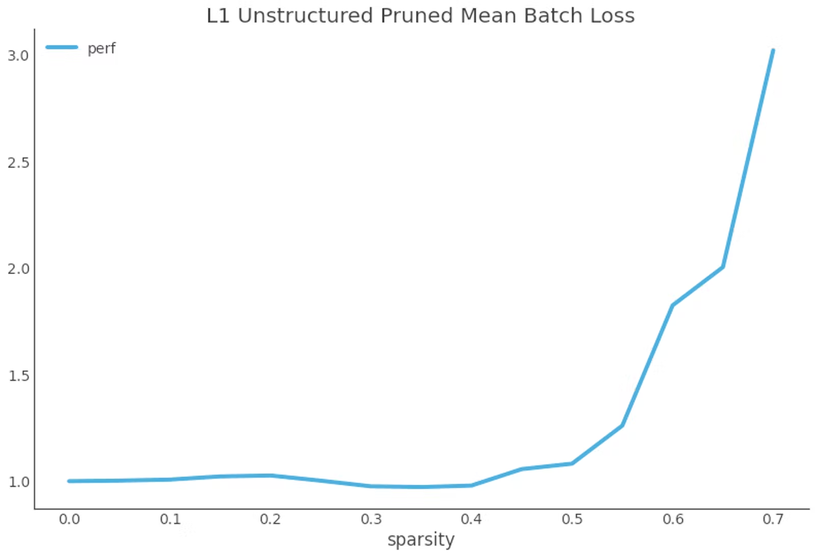
In this plot, 1 is the baseline (unpruned) model performance, and the other numbers are multiple of that baseline. So at 0.7, 70% sparsity, our loss is 3 times as high as it is for our baseline unpruned model.
Interpreting this plot, we see that approximately 40 to 50 percent of the Conv2d parameters in the model are purely noise, contributing no meaningful value to the overall prediction. These values can safely be pruned without affecting model inference. Past that point, our model loss grows exponentially—hence in this case.
This loss curve is extremely typical of model pruning performance. The placement of the “soft cap” on model sparsity is architecture-dependent, but the curve will always be exponential.
Next, let’s try structured pruning:
def prune_model_l1_structured(model, layer_type, proportion):
    for module in model.enc.modules():
        if isinstance(module, layer_type):
            prune.ln_structured(module, 'weight', proportion, n=1, dim=1)
            prune.remove(module, 'weight')
    return model
This code sample implements L1 structured pruning on the output channels dimensions: e.g. it removes proportion lowest-scoring channels (filters) from the Conv2d layer. Plotting the performance implications of L1 structured pruning, we get the following:
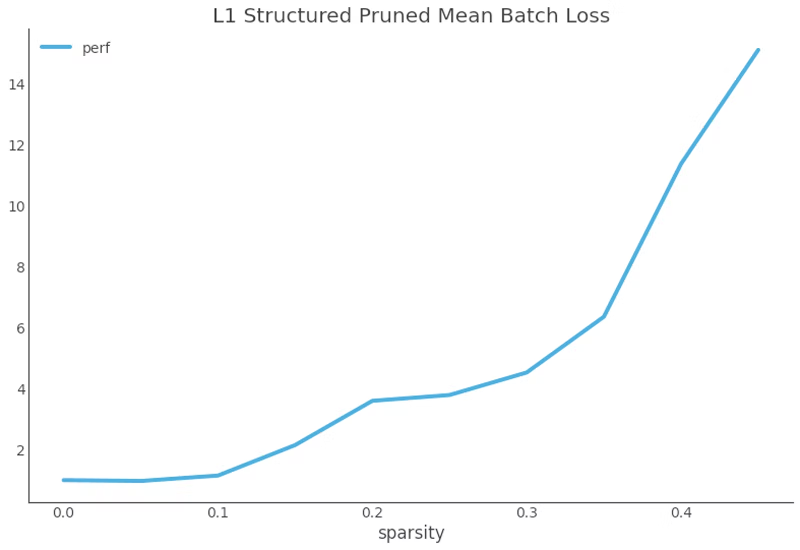
As you can see, structured pruning has much less fidelity than unstructured pruning. With our current implementation, we can only safely prune 5 to 10 percent of the model weights before performance begins to degrade. It appears that most of the filters in our model are doing something useful, and so we cannot remove them nearly as easily as we can individual weights.
This fits our intuition. While most of the features individual filters in a convolutional neural network look for will have areas which are sparse, and hence unimportant, a network which has been trained to convergence will hardly ever have an entire filter contributing only noise.
Let’s try one more pruning technique: global unstructured pruning. In global unstructured pruning, instead of specifying individual pruning parameters for individual layers, we apply to the model all at once. This allows us to prune less useful (lower entropy) layers more aggressively than more useful (higher entropy) ones.
The code:
def prune_model_global_unstructured(model, layer_type, proportion):
    module_tups = []
    for module in model.modules():
        if isinstance(module, layer_type):
            module_tups.append((module, 'weight'))

    prune.global_unstructured(
        parameters=module_tups, pruning_method=prune.L1Unstructured,
        amount=proportion
    )
    for module, _ in module_tups:
        prune.remove(module, 'weight')
    return model
The result:
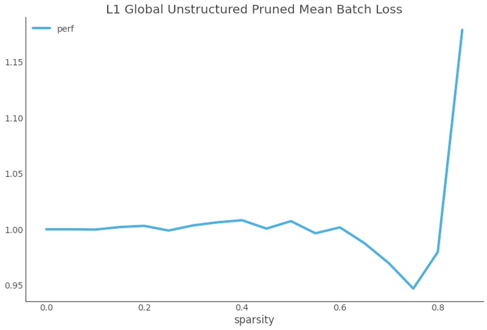
Taking a look at model performance we see that, remarkably, one-shot global unstructured pruning allows us to achieve 80 percent sparsity before model performance begins to degrade!
Effect on model size
Model pruning has a linear relationship with compressed model size. This is because compression algorithms are extremely efficient at serializing patterns containing strides of zeroes.
In deployment scenarios where on-disk size is important, e.g. model inference on edge devices, this is extremely useful.
Our model is 97 MB uncompressed, and 90 MB compressed with gzip (with default settings):
# in
model = get_model()
torch.save(model.state_dict(), "/tmp/model.h5")
!du -h /tmp/model.h5
!gzip -qf /tmp/model.h5
!du -h /tmp/model.h5.gz

# out
97M    /tmp/model.h5
90M    /tmp/model.h5.gz
After pruning the model to 40 percent sparsity, our model dips down to just 65 MB in size—a size reduction of 35%:
# in
model = get_model()
model = prune_model(model, nn.Conv2d, 0.4)
torch.save(model.state_dict(), "/tmp/model.h5")
!gzip -qf /tmp/model.h5
!du -h /tmp/model.h5.gz

# out
65M    /tmp/model.h5.gz