Data-Distributed Training
Contents
Data-Distributed Training
Distributed training is the set of techniques for training a deep learning model using multiple GPUs and/or multiple machines. Distributing training jobs allow you to push past the single-GPU memory and compute bottlenecks, expediting the training of larger models (or even making it possible to train them in the first place) by training across many GPUs simultaneously.
There are two types of distributed training that see use in production today. This chapter covers the better-known of the two techniques: data-distributed training. Data-distributed training works by initializing the same model on multiple different machines, slicing the batch up and backprogating on each machine simultaneously, collecting and averaging the resulting gradients, and then updating each local machine’s local copy of the model prior to the next round of training.
In native PyTorch this pattern is implemented by the torch.nn.parallel.DistributedDataParallel API.
You can follow along in code by checking out the companion GitHub repo.
TLDR: data-distributed training is the best way to train models too large to fit on disk on a single machine. However, the network synchronization required have a very real efficiency cost, so you should only turn to using this technique once you have exhausted your ability to scale your training instance vertically (e.g. you are already working with the largest GPU instance available to you).
Data parallelization versus model parallelization
A model training job that uses data parallelization is executed on multiple GPUs simultaneously. Each GPU in the job receives its own independent slice of the data batch (a batch slice), which it uses to independently calculate a gradient update. For example, if you were to use two GPUs and a batch size of 32, one GPU would handle forward and back propagation on the first 16 records, and the second the last 16. These gradient updates are then synchronized among the GPUs, averaged together, and finally applied to the model.
The synchronization step is technically optional, but theoretically faster asynchronous update strategies are still an active area of research.
Data parallelization competes with model parallelization for mindshare. In model parallelization, the model training job is split on the model. Each GPU in the job receives a slice of the model - a subset of its layers. So for example, one GPU might be responsible for its output head, another might handle the input layers, and still another the hidden layers in between.
Data parallelization (aka data-distributed training) is the easier of these two techniques to implement. It requires no knowledge of the underlying network architecture to implement and has robust API implementations.
This chapter will cover data-distributed training only. A future chapter covers model-distributed training. Note that it’s also possible to use these two techniques simultaneously.
How it works
As far as I can tell, the first data parallelization technique to see adoption in deep learning was the parameter server strategy in TensorFlow. This technique predates TensorFlow itself: it was actually first implemented in its Google-internal predecessor, DistBelief, in 2012. This strategy is illustrated in the following diagram (taken from here):
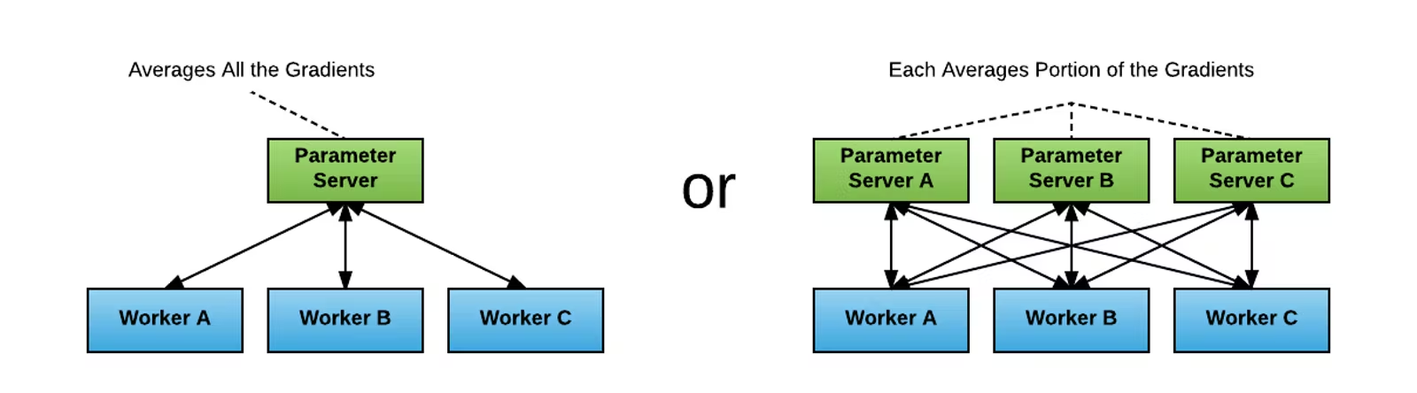
In the parameter server strategy there is a variable number of worker and parameter processes, with each worker process maintaining its own independent copy of the model in GPU memory. Gradient updates are computed as follows:
Upon receiving the go signal, each worker process accumulates the gradients for its particular batch slice.
The workers sends their update to the parameter servers in a fan-out manner.
The parameter servers wait until they have all worker updates, then average the total gradient for the portion of the gradient update parameter space they are responsible for.
The gradient updates are fanned out to the workers, which sum them up and apply them to their in-memory copy of the model weights (thus keeping the worker models in sync).
Once every worker has applied the updates, a new batch of training is ready to begin.
Whilst simple to implement, this strategy has some major limitations. Each additional parameter server requires n_workers additional network calls at each synchronization step — an O(n^2) complexity cost. Furthermore, computational sped was blocked on the slowest connection in the network. Large parameter server model training jobs proved to be very inefficient in practice, pushing net GPU utilization to 50% or below.
For the curious, the Inside TensorFlow: tf.distribute.Strategy tech talk has more details.
The 2017 Baidu paper Bringing HPC Techniques to Deep Learning improved upon this strategy. This paper experimentally validated a new distributed training strategy that did away with the parameter server component.
In this strategy, every process is a worker process. Each process still maintains a complete in-memory copy of the model weights, but batch slice gradients updates are now synchronized and averaged directly on the worker processes themselves. This is achieved using a technique borrowed from the high-performance computing world: an all-reduce algorithm:
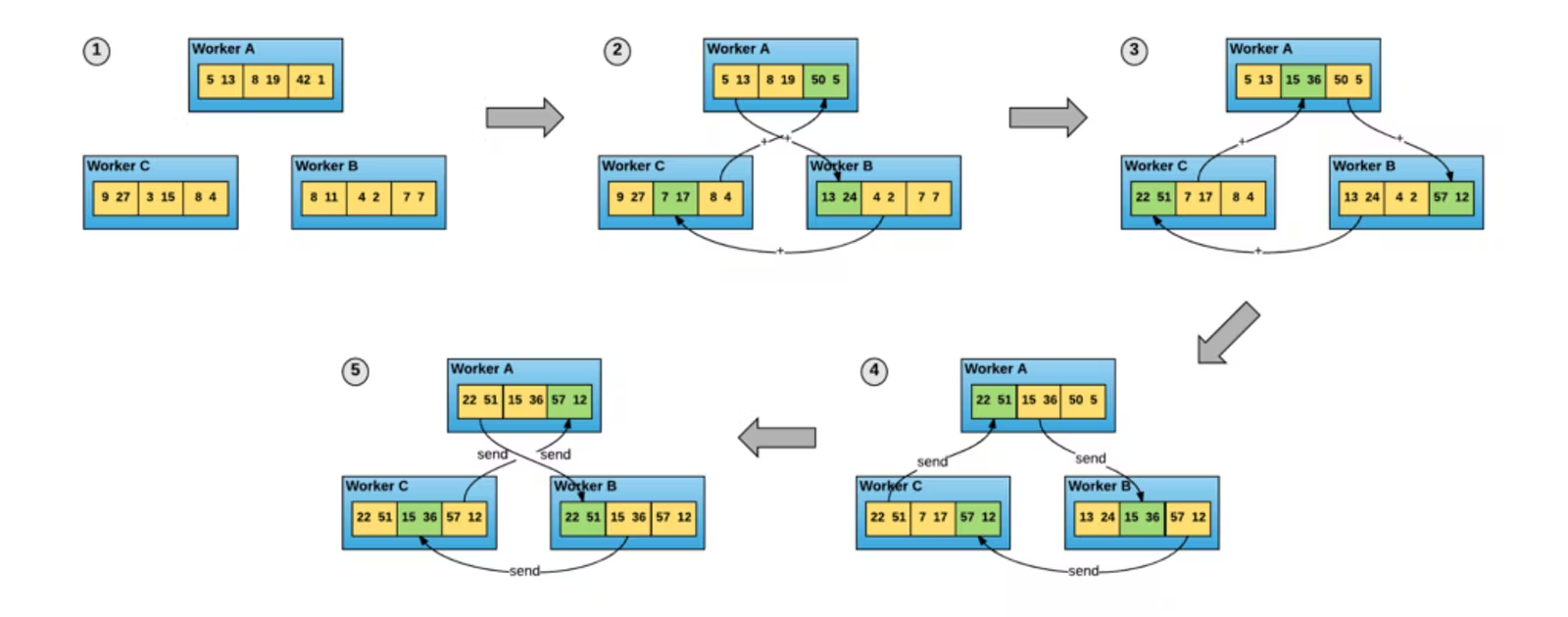
This diagram shows one particular implementation of an all-reduce algorithm, ring all-reduce, in action. The algorithm provides an elegant way of synchronizing the state of a set of tensors among a collection of processes. The tensors are passed in a ring (hence the name) by a sequence of direct worker-to-woker connections. This eliminates the network bottleneck created by the worker-to-parameter-server connections, substantially improving performance.
In this scheme, gradient updates are computed as follows:
Each worker maintains its own copy of the model weights and its own copy of the dataset.
Upon receiving the go signal, each worker process draws a disjoint batch from the dataset and computes a gradient for that batch.
The workers use an all-reduce algorithm to synchronize their individual gradients, computing the same average gradient on all nodes locally.
Each worker applies the gradient update to its local copy of the model.
The next batch of training is ready to begin.
The torch.nn.parallel.DistributedDataParallel PyTorch API is an implementation of this strategy.
The great thing about this approach is that all-reduce is a well-understood HPC techniques with longstanding open source implementations. All-reduce is part of the Message Passing Interface (MPI) de facto standard, which is why PyTorch DistributedDataParallel offfers not one but three different backends: Open MPI, NVIDIA NCCL, and Facebook Gloo.
Data distributed, part 1: process initialization
To demonstrate how the API works, we will build our way towards a complete distributed training script (which we will benchmark later). Here is the code on GitHub.
The first and most complicated new thing you need to handle is process initialization. A vanilla PyTorch training script executes a single copy of its code inside of a single process. With parallelized training, the situation is more complicated: there are now as many simultaneous copies of the training script as there are GPUs in the training cluster, each one running in a different process.
Consider the following minimal example:
# multi_init.py
import torch
import torch.distributed as dist
import torch.multiprocessing as mp

def init_process(rank, size, backend='gloo'):
    """ Initialize the distributed environment. """
    os.environ['MASTER_ADDR'] = '127.0.0.1'
    os.environ['MASTER_PORT'] = '29500'
    dist.init_process_group(backend, rank=rank, world_size=size)

def train(rank, num_epochs, world_size):
    init_process(rank, world_size)
    print(
        f"Rank {rank + 1}/{world_size} process initialized.\n"
    )
    # rest of the training script goes here!

WORLD_SIZE = torch.cuda.device_count()
if __name__=="__main__":
    mp.spawn(
        train, args=(NUM_EPOCHS, WORLD_SIZE),
        nprocs=WORLD_SIZE, join=True
    )
In the world of MPI, world size is the number of processes being orchestrated, and (global) rank is the position of the current process in that world. So for example, if this script were to be executing on a beefy machine with four GPUs onboard, WORLD_SIZE would be 4 (because torch.cuda.device_count() == 4), so mp.spawn would spawn 4 different processes, whose rank would be 0, 1, 2, or 3 respectively. The process with rank 0 is given a few extra responsibilities, and is therefore referred to as the master process.
The current process’s rank is passed through to the spawn entrypoint (in this case, the train method) as its first argument. Before train can actually do any work, it needs to first set up its connections to its peer processes. This is the responsibility of the dist.init_process_group. When run in the master process, this method sets up a socket listener on MASTER_ADDR:MASTER_PORT and starts handling connections from the other processes. Once all of the processes have connected, this method handles setting up the peer connections allowing the processes to communicate.
Note that this recipe only works for training on a single multi-GPU machine! The same machine is used to launch every single process in the job, so training can only leverage the GPUs connected to that specific machine. This makes things easy: setting up IPC is as easy as finding a free port on localhost, which is immediately visible to all processes on that machine. IPC across machines is more complicated, as it requires configuring an external IP address visible to all machines.
In this introductory tutorial we will focus specifically on the single-machine case, aka vertical scaling. Even on its own, vertical scaling is an extremely powerful tool. On the cloud, vertical scaling allows you to scale your deep learning training job all the way up to an A100x8. That’s a lot of deep learning horsepower!
We will discuss horizontal scaling with data parallelization in a future blog post. In the meantime, to see a code recipe showing it in action, check out the PyTorch AWS tutorial.
Data distributed, part 2: process synchronization
Now that we understand the initialization process, we can start filling out the body of the train method that does all of the work.
Recall what we have so far:
def train(rank, num_epochs, world_size):
    init_process(rank, world_size)
    print(
        f"{rank + 1}/{world_size} process initialized.\n"
    )
    # rest of the training script goes here!
Each of our four training processes runs this function to completion, exiting out when it is finished. If we were to run this code right now (via python multi_init.py), we would see something like the following printed out to our console:
$ python multi_init.py
1/4 process initialized.
3/4 process initialized.
2/4 process initialized.
4/4 process initialized.
The processes are independently executed, and there are no guarantees about what state any one state is at any one point in the training loop. This requires making some careful changes to your initialization process.
(1) Any methods that download data should be isolated to the master process.
Failing to do so will replicate the download process across all of the processes, resulting in four processes writing to the same file simultaneously, wasting a lot of time and possibly risking a filesystem deadlock. This can be done as follows:
# import torch.distributed as dist
if rank == 0:
    downloading_dataset()
    downloading_model_weights()
dist.barrier()
print(
    f"Rank {rank + 1}/{world_size} training process passed data download barrier.\n"
)
The dist.barrier call in this code sample will block until the master process (rank == 0) is done downloading_dataset and downloading_model_weights. This isolates all of the network I/O to a single process and prevents the other processes from jumping ahead until it’s done.
(2) The data loader needs to use DistributedSampler. Code sample:
def get_dataloader(rank, world_size):
    dataset = PascalVOCSegmentationDataset()
    sampler = DistributedSampler(
        dataset, rank=rank, num_replicas=world_size, shuffle=True
    )
    dataloader = DataLoader(
        dataset, batch_size=8, sampler=sampler
    )
DistributedSampler uses rank and world_size to partition the dataset across the processes into non-overlapping batches. Every training step the worker process retrieves batch_size observations from its local copy of the dataset. In the example case of four GPUs, this means an effective batch size of 8 * 4 = 32.
(3) Tensors needs to be loaded into the correct device. To do so, parameterize your .cuda() or .to() calls with the rank of the device the process is managing:
batch = batch.cuda(rank)
segmap = segmap.cuda(rank)
model = model.cuda(rank)
(4) Any randomness in model initialization must be disabled.
It’s extremely important that the models start and remain synchronized throughout the entire training process. Otherwise, you’ll get inaccurate gradients and the model will fail to converge.
Random initialization methods like torch.nn.init.kaiming_normal_ can be made deterministic using the following code:
torch.manual_seed(0)
torch.backends.cudnn.deterministic = True
torch.backends.cudnn.benchmark = False
np.random.seed(0)
The PyTorch documentation has an entire Reproducibility page dedicated to this topic.
(5) Any methods that perform file I/O should be isolated to the master process.
This is necessary for the same reason that isolating network I/O is necessary: the inefficiency and potential for data corruption created by concurrent writes to the same file. Again, this is easy to do using simple conditional logic:
if rank == 0:
    if not os.path.exists('/spell/checkpoints/'):
        os.mkdir('/spell/checkpoints/')
        torch.save(
            model.state_dict(),
            f'/spell/checkpoints/model_{epoch}.pth'
        )
As an aside, note that any global loss values or statistics you want to log will require you to synchronize the data yourself. This can be done using additional MPI primitives in torch.distributed not covered in-depth in this tutorial. Check out this gist I prepared for a quick intro, and refer to the Distributed Communication Package PyTorch docs page for a detailed API reference.
(6) The model must be wrapped in DistributedDataParallel.
Assuming you’ve done everything else correctly, this is where the magic happens. ✨
model = DistributedDataParallel(model, device_ids=[rank])
With that change the model is now training in distributed data parallel mode!
What about DataParallel?
Readers familiar with the PyTorch API may know that there is also one other data parallelization strategy in PyTorch, torch.nn.DataParallel. This API is much easier to use; all you have to do is wrap your model initialization like so:
model = nn.DataParallel(model)
A one-liner change! Why not just use that instead?
Under the hood, DataParallel uses multithreading, instead of multiprocessing, to manage its GPU worker. This greatly simplifies the implementation: since the workers are all different threads of the same process, they all have access to the same shared state without requiring any additional synchronization steps.
However, using multithreading for computational jobs in Python is famously unperformant, due to the presence of the Global Interpreter Lock. As the benchmarks in the next section will show, models parallelized using DataParallel are significantly slower than those parallelized using DistributedDataParallel.
Benchmarks
To benchmark distributed model training performance I trained a DeepLabV3-ResNet 101 model (via Torch Hub) on the PASCAL VOC 2012 dataset (from torchvision datasets) for 20 epochs. I used the Spell API to launch five different versions of this model training job: once on a single V100 (a p3.2xlarge on AWS), and once each on a V100x4 (p3.8xlarge) and a V100x8 (p3.16xlarge) using DistributedDataParallel and DataParallel. This benchmark excludes the time spent downloading data at the beginning of the run—only model training and saving time counts.
The results are not definitive by any means, but should nevertheless give you some sense of the time save distributed training nets you:
Author note: these benchmarks were last run in June 2020. Improvements in the DistributedDataParallel implementation have likely further reduced runtimes since then.
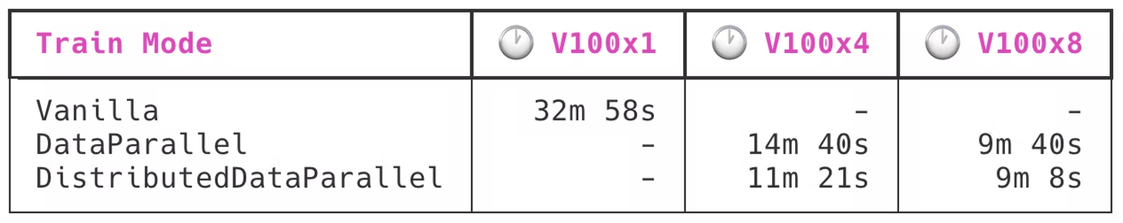
As you can clearly see, DistributedDataParallel is noticeably more efficient than DataParallel, but still far from perfect. Switching from a V100x1 to a V100x4 is a 4x multiplier on raw GPU power but only 3x on model training speed. Doubling the compute further by moving up to a V100x8 only produces a ~30% improvement in training speed. By that point DataParallel almost catches up to DistributedDataParallel in (in)efficiency.
Note that this is still an active area of development. Expect these times to continue to improve in new PyTorch releases!